Introduction

Why generative modeling?

Before we start thinking about (deep) generative modeling, let us consider a simple example. Imagine we have trained a deep neural network that classifies images ($\mathbf{x} \in \mathbb{Z}^{D}$) of animals ($y \in \mathcal{Y}$, and $\mathcal{Y} = \{cat, dog, horse\}$). Further, let us assume that this neural network is trained well so that it always classifies a proper class with a high probability $p(y|\mathbf{x})$. However, (Szegedy et al., 2013) pointed out that adding noise to images could result in completely false classification. An example of such a situation is presented in Figure 1 where adding noise could shift predicted probabilities of labels, however, the image is barely changed.

Figure 1. An example of adding noise to an almost perfectly classified image that results in a shift of predicted label.

This example indicates that neural networks that are used to parameterize the conditional distribution $p(y|\mathbf{x})$ lack semantic understanding of images. Further, we even hypothesize that learning discriminative models is not enough for proper decision making and creating AI. A machine learning system cannot rely on learning how to make a decision without understanding the reality and being able to express uncertainty about the surrounding world. How can we trust such a system if even a small amount of noise could change its internal beliefs, and also shift its certainty from one decision to the other? How can we communicate with such a system if it is unable to properly express its opinion about whether its surrounding is new or not?

To motivate the importance of the concepts like uncertainty and understanding in decision making, let us consider a system that classifies objects, but this time into two classes: orange and blue. We assume we have some two-dimensional data (Figure 2, left) and a new datapoint to be classified (a black cross in Figure 2). We can make decisions using two approaches. First, a classifier could be formulated explicitly by modeling the conditional distribution $p(y|\mathbf{x})$ (Figure 2, middle). Second, we can consider a joint distribution $p(\mathbf{x}, y)$ that could be further decomposed as $p(\mathbf{x}, y) = p(y|\mathbf{x})\ p(\mathbf{x})$ (Figure 2, right).

Figure 2 And example of data (left) and two approaches to decision making: (middle) a discriminative approach, (right) a generative approach.

After training a model using the discriminative approach, namely, the conditional distribution $p(y|\mathbf{x})$, we obtain a clear decision boundary. Then, we see that the black cross is farther away from the orange region, thus, the classifier assigns a higher probability to the blue label. As a result, the classifier is certain about the decision!

On the other hand, if we additionally fit a distribution $p(\mathbf{x})$, we observe that the black cross is not only farther away from the decision boundary, but also it is distant to the region where blue datapoints lie. In other words, the black point is far away from the region of high probability mass. As a result, the probability of the black cross, $p(\mathbf{x}=black\ cross)$ is low, and the joint distribution $p(\mathbf{x}= black\ cross, y=blue)$ will be low as well and, thus, the decision is uncertain!

This simple example clearly indicates that if we want to build AI systems that make reliable decisions and can communicate with us, human beings, they must understand the environment first. For this purpose, they cannot simply learn how to make decisions, but they should be able to quantify their beliefs about their surrounding using the language of probability (Bishop, 2013; Ghahramani, 2015). In order to do that, we claim that estimating the distribution over objects, $p(\mathbf{x})$, is crucial.

From the generative perspective, knowing the distribution $p(\mathbf{x})$ is a essential because:

• it could be used to assess whether a given object has been observed in the past or not;
• it could help to properly weight the decision;
• it could be used to assess uncertainty about the environment;
• it could be used to actively learn by interacting with the environment (e.g., by asking for labeling objects with low $p(\mathbf{x})$);
• and, eventually, it could be used to generate new objects.

Typically, in the literature of deep learning, generative models are treated as generators of new data. However, here we try to convey a new perspective where having $p(\mathbf{x})$ has much broader applicability, and this could be essential for building successful AI systems. Lastly, we would like to also make an obvious connection to generative modeling in machine learning, where formulating a proper generative process is crucial for understanding the phenomena of interest (Lasserre et al., 2006). However, in many cases, it is easier to focus on the other factorization, namely, $p(\mathbf{x}, y) = p(\mathbf{x}|y)\ p(y)$. We claim that considering $p(\mathbf{x}, y) = p(y|\mathbf{x})\ p(\mathbf{x})$ has clear advantages as mentioned before.

Where can we use (deep) generative modeling?

With the development of neural networks and increase computational power, deep generative modeling become one of the leading directions in AI. Its applications vary from typical modalities considered in machine learning, i.e., text analysis (Bowman et al., 2015), image analysis (Goodfellow et al., 2014), audio analysis (v.d. Oord et al., 2016a), to problems in active learning (Sinha et al., 2019), reinforcement learning (Ha & Schmidhuber, 2018), graph analysis (Simonovsky & Komodakis, 2018) and medical imaging (Ilse et al., 2020). In Figure 3, we present graphically potential applications of deep generative modeling.

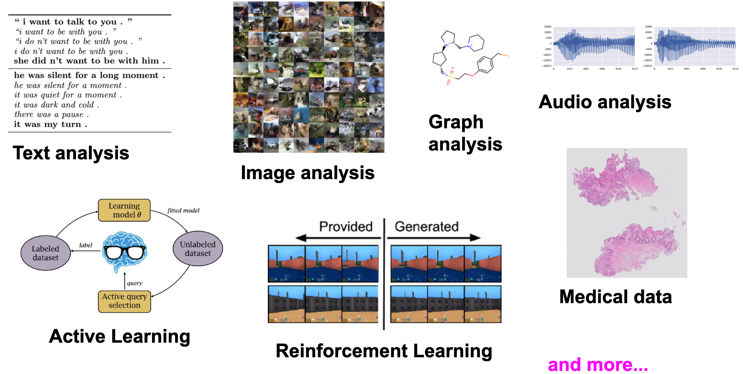
Figure 3. Various applications of deep generative modeling.

In some applications, it is indeed important to generate objects or modify features of objects to create new ones (e.g., an app turns a young person into an old one). However, in active learning it is important to ask for uncertain objects (i.e., with low $p(\mathbf{x})$) that should be labeled by an oracle. In reinforcement learning, on the other hand, generating the next most likely situation (states) is crucial for taking actions by an agent. For medical applications, explaining a decision, e.g., in terms of the probability of the label and the object, is definitely more informative to a human doctor than simply assisting with a diagnosis label. If an AI system would be able to indicate how certain it is, and also quantify whether the object is suspicious (i.e., low $p(\mathbf{x})$) or not, then it might be used as an independent specialist that outlines its own opinion.

These examples clearly indicate that many fields, if not all, could highly benefit from (deep) generative modeling. Obviously, there are many mechanisms that AI systems should be equipped with. However, we claim that the generative modeling capability is definitely one of the most important ones, as outlined in the abovementioned cases.

How to formulate (deep) generative modeling?

At this point, after highlighting the importance and wide applicability of (deep) generative modeling, we should ask ourselves how to formulate (deep) generative models. In other words, how to express $p(\mathbf{x})$ that we mentioned already multiple times.

We can divide (deep) generative modeling into three main groups (see Figure 4):

• autoregressive generative models (ARM);
• flow-based models;
• latent variable models.

We use deep in brackets because most of what we have discussed so far could be modeled without using neural networks. However, neural networks are flexible and powerful, therefore, they are widely used to parameterize generative models. From now on, we focus entirely on deep generative models.

As a side note, we would like to mention that there are other deep generative models, e.g., energy-based models (Hinton & Ghahramani, 1997) or recently proposed deep diffusion models (Ho et al., 2020). Here, we focus on the three groups that are most popular in the deep generative modeling literature.

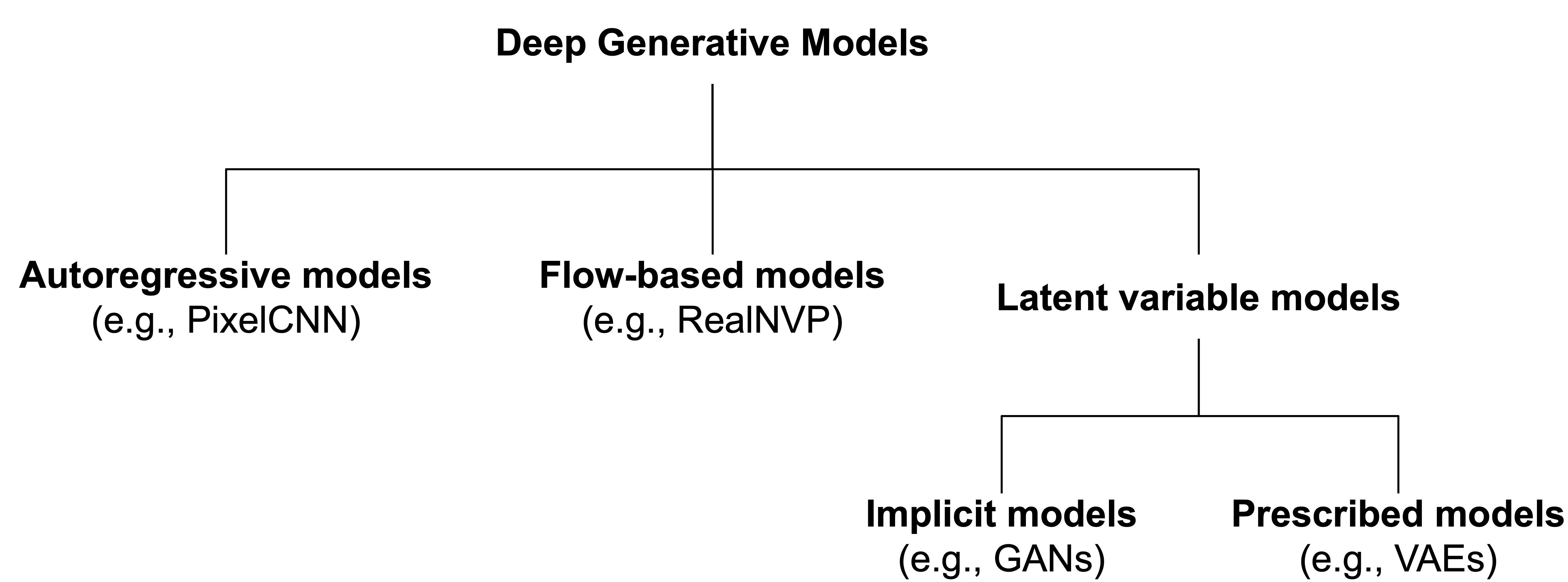
Figure 4. A diagram representing deep generative models.

Autoregressive models

The first group of deep generative models utilzes the idea of autoregressive modeling (ARM). In other words, the distribution over $\mathbf{x}$ is represented in an autoregresve manner: $$ p(\mathbf{x}) = p(x_0) \prod_{i=1}^{D} p(x_i|\mathbf{x}_{<i}), $$ where $\mathbf{x}_{<i}$ denotes all $\mathbf{x}$'s up to the index $i$.

Modeling all conditional distributions $p(x_i|\mathbf{x}_{<i})$ would be computationally inefficient. However, we can take advantage of causal convolutions as presented in (v.d. Oord et al., 2016a) for audio, and in (v.d. Oord et al., 2016b) for images.

Flow-based models

The change of variables formula provides a principled manner of expressing a density of a random variable by transforming it with an invertible transformation $f$ (Rippel & Adams, 2013): $$ p(\mathbf{x}) = p\big{(}\mathbf{z} = f(\mathbf{x})\big{)} |\mathbf{J}_{f(\mathbf{x})}| $$ where $\mathbf{J}_{f(\mathbf{x})}$ denotes the Jacobian matrix.

We can parameterize $f$ using deep neural networks, however, it cannot be any arbitrary neural networks, because we must be able to calculate the Jacobian matrix. First attempts focused on linear transformations that are volume-preserving that yields $|\mathbf{J}_{f(\mathbf{x})}|=1$ (Dinh et al., 2014; Tomczak & Welling, 2016). Further attempts utilized theorems on matrix determinants that resulted in specific non-linear transformations, namely, planar flows (Rezende & Mohamed, 2015), and Sylvester flows (van den Berg et al., 2018; Hoogeboom et al., 2020). A different approach focuses on formulating invertible transformations for which the Jacobian-determinant could be calculated easily like for coupling layers in RealNVP (Dinh et al., 2016).

In the case of the discrete distributions (e.g., integers), for the probability mass functions, there is no change of volume, therefore, the change of variable formulate takes the following form: $$ p(\mathbf{x}) = p\big{(}\mathbf{z} = f(\mathbf{x})\big{)}. $$

Integer discrete flows propose to use affine coupling layers with rounding operators to ensure the integer-valued output (Hoogeboom et al., 2019). A generalization of the affine coupling layer was further investigated in (Tomczak, 2020).

All generative models that take advantage of the change of variables formula are referred to as flow-based models.

Latent variable models

The idea behind latent variable models is to assume a lower-dimensional latent space and the following generative process: \begin{align*} \mathbf{z} &\sim p(\mathbf{z}) \\ \mathbf{x} &\sim p(\mathbf{x}|\mathbf{z}) . \end{align*} In other words, the latent variables correspond to hidden factors in data, and the conditionl distribution $p(\mathbf{x}|\mathbf{z})$ could be treated as a generator.

The most widely-known latent variable model is the probabilistic Principal Analysis (pPCA) (Tipping & Bishop, 1999) where $p(\mathbf{z})$ and $p(\mathbf{x}|\mathbf{z})$ are Gaussian distributions, and the dependency between $\mathbf{z}$ and $\mathbf{x}$ is linear.

A non-linear extension of the pPCA with arbitrary distributions is the Variational Auto-Encoder (VAE) framework (Kingma & Welling, 2013; Rezende et al., 2014). To make the inference tractable, variational inference is utilized to approximate the posterior $q(\mathbf{z}|\mathbf{x})$, and neural networks are used to parameterize the distributions. Since the seminal papers by Kingma & Welling, and Rezende et al., there were multiple extensions of the framework, including working on more powerful variational posteriors (van den Berg et al., 2018; Kingma et al., 2016; Tomczak & Welling, 2016), priors (Tomczak & Welling, 2018) and decoders (Gulrajani et al., 2016). Interesting directions include also considering different topologies of the latent space, e.g., the hyperspherical latent space (Davidson et al., 2018). In VAEs and the pPCA all distributions must be defined upfront, therefore, they are called prescribed models.

So far, ARMs, flows, the pPCA, and VAEs are probabilistic models with the objective function being the log-likelihood function that is closely related to using the Kullback-Leibler divergence between the data distribution and the model distribution. A different approach utilizes and adversarial loss in which a discriminator $D(\cdot)$ determines a difference between real data and data provided by a generator in the implicit form, namely, $p(\mathbf{x}|\mathbf{z}) = \delta\big{(}\mathbf{x} - G(\mathbf{z})\big{)}$, where $\delta(\cdot)$ is the Dirac delta. This group of models is called implicit models and Generative Adversarial Networks (GANs) (Goodfellow et al., 2014) become one of the most successful deep generative models for generating realistic-looking objects (e.g., images).

Overview

In Table 1, we compared all three groups of models (with a distinction between implicit latent variable models and prescribed latent variable models) using arbitrary criteria like training stability, ability to calculate the likelihood function and direct applicability to lossy or lossless compression.

All likelihood-based models (i.e., ARMs, flows, and prescribed models like VAEs) can be trained stably while implicit models like GANs suffer from instabilities. In the case of the non-linear prescribed models like VAEs, we must remember that the likelihood function cannot be exactly calculated, and only a lower-bound could be provided. ARMs constitute one of the best likelihood-based models, however, their sampling process is extremely slow due to the autoregressive manner of generating new content. All other approaches are relatively fast. In the case of lossy compression, VAEs are models that allow us to use a bottleneck (the latent space). On the other hand, ARMs and flows could be used for lossless compression since they are density estimators and provide the exact likelihood value. Implicit models cannot be directly used for compression, however, recent works use GANs to improve image compression.

Table 1. A comparison of deep generative models.

Generative models	Training	Likelihood	Sampling	Lossy compression	Lossless compression
Autoregressive models	stable	exact	slow	no	yes
Flow-based models	stable	exact	fast/slow	no	yes
Implicit models	unstable	no	fast	no	no
Prescribed model	stable	approximate	fast	yes	no

References

(Bauer & Mnih, 2019) Bauer, Matthias, and Andriy Mnih. "Resampled priors for variational autoencoders." In The 22nd International Conference on Artificial Intelligence and Statistics, pp. 66-75. PMLR, 2019.

(van den Berg et al., 2018) van den Berg, Rianne, Leonard Hasenclever, Jakub M. Tomczak, and Max Welling. "Sylvester normalizing flows for variational inference." In 34th Conference on Uncertainty in Artificial Intelligence 2018, UAI 2018, pp. 393-402. Association For Uncertainty in Artificial Intelligence (AUAI), 2018.

(Bishop, 2013) Bishop, Christopher M. "Model-based machine learning." Philosophical Transactions of the Royal Society A: Mathematical, Physical and Engineering Sciences 371, no. 1984 (2013).

(Bowman et al., 2015) Bowman, Samuel R., Luke Vilnis, Oriol Vinyals, Andrew M. Dai, Rafal Jozefowicz, and Samy Bengio. "Generating sentences from a continuous space." arXiv preprint arXiv:1511.06349 (2015).

(Davidson et al., 2018) Davidson, Tim R., Luca Falorsi, Nicola De Cao, Thomas Kipf, and Jakub M. Tomczak. "Hyperspherical variational auto-encoders." In 34th Conference on Uncertainty in Artificial Intelligence 2018, UAI 2018, pp. 856-865. Association For Uncertainty in Artificial Intelligence (AUAI), 2018.

(Dinh et al., 2014) Dinh, Laurent, David Krueger, and Yoshua Bengio. "NICE: Non-linear independent components estimation." arXiv preprint arXiv:1410.8516 (2014).

(Dinh et al., 2016) Dinh, Laurent, Jascha Sohl-Dickstein, and Samy Bengio. "Density estimation using real nvp." arXiv preprint arXiv:1605.08803 (2016).

(Ghahramani, 2015) Ghahramani, Zoubin. "Probabilistic machine learning and artificial intelligence." Nature 521, no. 7553 (2015): 452-459.

(Goodfellow et al., 2014) Goodfellow, Ian, Jean Pouget-Abadie, Mehdi Mirza, Bing Xu, David Warde-Farley, Sherjil Ozair, Aaron Courville, and Yoshua Bengio. "Generative adversarial nets." In Advances in neural information processing systems, pp. 2672-2680. (2014).

(Gulrajani et al., 2016) Gulrajani, Ishaan, Kundan Kumar, Faruk Ahmed, Adrien Ali Taiga, Francesco Visin, David Vazquez, and Aaron Courville. "PixelVAE: A latent variable model for natural images." arXiv preprint arXiv:1611.05013 (2016).

(Ha & Schmidhuber, 2018) Ha, David, and Jurgen Schmidhuber. "World models." arXiv preprint arXiv:1803.10122 (2018).

(Hinton & Ghahramani, 1997) Hinton, Geoffrey E., and Zoubin Ghahramani. "Generative models for discovering sparse distributed representations." Philosophical Transactions of the Royal Society of London. Series B: Biological Sciences 352, no. 1358 (1997): 1177-1190.

(Ho et al., 2020) Ho, Jonathan, Ajay Jain, and Pieter Abbeel. "Denoising diffusion probabilistic models." Advances in Neural Information Processing Systems 33 (2020).

(Hoogeboom et al., 2019) Hoogeboom, Emiel, Jorn Peters, Rianne van den Berg, and Max Welling. "Integer discrete flows and lossless compression." In Advances in Neural Information Processing Systems, pp. 12134-12144. 2019.

(Hoogeboom et al., 2020) Hoogeboom, Emiel, Victor Garcia Satorras, Jakub M. Tomczak, and Max Welling. "The Convolution Exponential and Generalized Sylvester Flows." arXiv preprint arXiv:2006.01910 (2020).

(Ilse et al., 2020) Ilse, Maximilian, Jakub M. Tomczak, Christos Louizos, and Max Welling. "DIVA: Domain invariant variational autoencoders." In Medical Imaging with Deep Learning, pp. 322-348. PMLR, 2020.

(Kingma & Welling, 2013) Kingma, Diederik P., and Max Welling. "Auto-encoding variational bayes." arXiv preprint arXiv:1312.6114 (2013).

(Kingma et al., 2016) Kingma, Durk P., Tim Salimans, Rafal Jozefowicz, Xi Chen, Ilya Sutskever, and Max Welling. "Improved variational inference with inverse autoregressive flow." Advances in neural information processing systems 29 (2016): 4743-4751.

(Lasserre et al., 2006) Lasserre, Julia A., Christopher M. Bishop, and Thomas P. Minka. "Principled hybrids of generative and discriminative models." In 2006 IEEE Computer Society Conference on Computer Vision and Pattern Recognition (CVPR'06), vol. 1, pp. 87-94. IEEE, 2006.

(v.d. Oord et al., 2016a) van den Oord, Aaron, Sander Dieleman, Heiga Zen, Karen Simonyan, Oriol Vinyals, Alex Graves, Nal Kalchbrenner, Andrew Senior, and Koray Kavukcuoglu. "Wavenet: A generative model for raw audio." arXiv preprint arXiv:1609.03499 (2016).

(v.d. Oord et al., 2016b) van Den Oord, Aaron, Nal Kalchbrenner, and Koray Kavukcuoglu. "Pixel recurrent neural networks." In Proceedings of the 33rd International Conference on International Conference on Machine Learning-Volume 48, pp. 1747-1756. (2016).

(Rezende et al., 2013) Rezende, Danilo Jimenez, Shakir Mohamed, and Daan Wierstra. "Stochastic backpropagation and approximate inference in deep generative models." arXiv preprint arXiv:1401.4082 (2014).

(Rezende & Mohamed, 2015) Rezende, Danilo Jimenez, and Shakir Mohamed. "Variational inference with normalizing flows." arXiv preprint arXiv:1505.05770 (2015).

(Rippel & Adams, 2013) Rippel, Oren, and Ryan Prescott Adams. "High-dimensional probability estimation with deep density models." arXiv preprint arXiv:1302.5125 (2013).

(Simonovsky & Komodakis, 2018) Simonovsky, Martin, and Nikos Komodakis. "Graphvae: Towards generation of small graphs using variational autoencoders." In International Conference on Artificial Neural Networks, pp. 412-422. Springer, Cham, 2018.

(Sinha et al., 2019) Sinha, Samarth, Sayna Ebrahimi, and Trevor Darrell. "Variational adversarial active learning." In Proceedings of the IEEE International Conference on Computer Vision, pp. 5972-5981. 2019.

(Szegedy et al., 2013) Szegedy, Christian, Wojciech Zaremba, Ilya Sutskever, Joan Bruna, Dumitru Erhan, Ian Goodfellow, and Rob Fergus. "Intriguing properties of neural networks." arXiv preprint arXiv:1312.6199 (2013).

(Tipping & Bishop, 1999) Tipping, Michael E., and Christopher M. Bishop. "Probabilistic principal component analysis." Journal of the Royal Statistical Society: Series B (Statistical Methodology) 61, no. 3 (1999): 611-622.

(Tomczak & Welling, 2016) Tomczak, Jakub M., and Max Welling. "Improving variational auto-encoders using householder flow." arXiv preprint arXiv:1611.09630 (2016).

(Tomczak & Welling, 2018) Tomczak, Jakub, and Max Welling. "VAE with a VampPrior." In International Conference on Artificial Intelligence and Statistics, pp. 1214-1223. PMLR, 2018.

(Tomczak, 2020) Tomczak, Jakub M. "General Invertible Transformations for Flow-based Generative Modeling." arXiv preprint arXiv:2011.15056 (2020).