Score-based generative models: Score matching

Introduction

Let us start with the following quote from the abstract of (Song et al., 2020):

"Creating noise from data is easy; creating data from noise is generative modeling."

I must say that it is hard to come up with a shorter definition of concurrent generative modeling. Once we look at various classes of models, we immediately notice that this is exactly what we try to do: Generate data from noise! Don't believe me? OK, we should have a look at how various classes of generative models work:

• GANs: Sample noise $\mathbf{z}$ from a known $p(\mathbf{z})$ and use a generator $G(\mathbf{z})$ to get data.
• VAEs: Sample noise $\mathbf{z}$ from a prior $p(\mathbf{z})$ and use a decoder $p(\mathbf{x} | \mathbf{z})$ to sample data.
• Normalizing flows: Sample noise $\mathbf{z}$ from a base distribution $p(\mathbf{z})$ and use an invertible transformation $f$ to get data, $\mathbf{x} = f^{-1}(\mathbf{z})$.

I hope you see the pattern, my curious reader. In general, we can say that we look for a tranformation $\psi$ that maps noise $\mathbf{z}$ to data $\mathbf{x}$, namely, $\mathbf{x} = \psi(\mathbf{z})$. An example is presented in Figure 1.

Figure 1. A schematic representation of generative modeling seen as mapping noise (left: black crosses) to data (right: black crosses around orange moons) using some transformation $\psi$.

In GANs, VAEs and normalizing flows, the transformation is done in a "single step" by some neural net, namely, noise is mapped to data through a generator, a decoder or an inversion of $f$, respectively. However, this does not need to be accomplished in this manner. In fact, we could easily think of an iterative process. And we know such a class of models already: Diffusion-based models! The forward diffusion adds Gaussian noise to a data point in the consecutive steps until the data point becomes pure Gaussian noise, i.e., $\mathbf{x}_0 \sim p_{data}(\mathbf{x})$ and $\mathbf{x}_1 \sim \mathcal{N}(0, \mathbf{I})$ (a notation reminder: a datapoint $\mathbf{x} \equiv \mathbf{x}_0$ and noise $\mathbf{z} \equiv \mathbf{x}_1$). Then, the generative part (a.k.a. the backward diffusion) starts with $\mathbf{x}_1$ (i.e., pure Gaussian noise) and removes small amount of noise step-by-step until data $\mathbf{x}_0$ is achieved. In first implementations of diffusion models (Sohl-Dickstein et al., 2015; Ho et al., 2020), a finite number of steps was used, $T < +\infty$, thus, diffusion-based models could be seen as hierarchical VAEs with fixed encoders, see the post on diffusion models, and (Kingma et al., 2021).

In practice, the success of diffusion-based models comes from their depth, among other aspects (e.g., see the post on information-theoretic properties of diffusion models). In other words, we can learn extremely deep hierarchical models (e.g., $T=1000$) because the generation process is defined as removing small bits of noise for two consecutive variables. During training, a shared network is trained to predict this tiny-teeny amount of noise in a stochastic manner by sampling $t \in [0, 1]$ and then optimizing the following loss:

\begin{equation}\label{eq:diffusion_kl_t}\tag{1} \mathcal{L}_{t}(\mathbf{x}_{t}) = \mathbb{E}_{\mathcal{N}(\epsilon | 0, \mathbf{I})} \left[\gamma_t \| \epsilon - \epsilon_{\theta}(\mathbf{x}_{t}, t) \|^{2} \right] , \end{equation}

where $\epsilon_t$ is a sample from the standard Gaussian, $\gamma_t$ is a variance following from the noise schedule, $\epsilon_{\theta}(\cdot)$ is a shared neural net across all $t$'s that aims at predictimg $\epsilon$ given $\mathbf{x}_{t}$ and $t$, and $\mathbf{x}_{t}$ could be expressed using given data $\mathbf{x}_0$ and $\epsilon$. For simplicity, $\gamma_t$ is set to $1$ that results in the so-called simplified objective (Ho et al., 2020), but it could be also learnt (Kingma & Gao, 2023).

I know you, my curious reader, and I see your question coming. Since diffusion models work so good because the number of steps $T$ being large, why we should not go wild and take infinitely many steps, $T = +\infty$. It is a reasonable way of thinking, nonetheless, it entails some issues. First, we would need to deal with continuous $t \in [0, 1]$. However, we actually know that we can use differential equations to take care of this issue. But then a second issue arises: How to define generative models through differential equations? Ideally, we would like to obtain a method that allows us to train such models in a simple way with a loss similar to (\ref{eq:diffusion_kl_t}). It turns out that it is possible! But first, we will look into a different way of changing noise to data, a method called score matching. After that, we will be equipped with a learning strategy for dealing with continuous time (i.e., infinitely deep generative models). Eventually, we will discuss an alternative to score matching called flow matching.

Score matching

Keep in mind that our goal is to propose a model that turns noise to data in an iterative manner. Here is our first attempt. Imagine the following situation:

• We have access to the real distribution $p_{real}(\mathbf{x})$, where $\mathbf{x} \in \mathcal{X}$.
• We take any point in the data space at random (e.g., we sample from a uniform distribution over $\mathcal{X}$), $\hat{\mathbf{x}} \in \mathcal{X}$. There is a very high chance that $p_{real}(\hat{\mathbf{x}})$ is close to $0$, $p_{real}(\hat{\mathbf{x}}) \approx 0$.
• The question is then this: How to turn $\hat{\mathbf{x}}$ into a legit data point (i.e., an object that could be observed in real life)?

Actually, there is a good (i.e., relatively fast and theoretically well-grounded) method called stochastic gradient Langevin dynamics (SGLD) a.k.a. Langevine dynamics (Welling & Teh, 2011) that allows to sample from $p_{real}(\mathbf{x})$. If we start in $\mathbf{x}_0 \equiv \hat{\mathbf{x}}$, then by following this procedure:

\begin{equation}\label{eq:sgld}\tag{2} \mathbf{x}_{t + \Delta} = \mathbf{x}_{t} + \alpha\ \nabla_{\mathbf{x}_{t}} \ln p_{real}(\mathbf{x}) + \eta \cdot \epsilon , \end{equation}

where $\Delta$ is an increment, $\alpha > 0$, $\eta > 0$, and $\epsilon \sim \mathcal{N}(0, \mathbf{I})$, we eventually end up in a point $\mathbf{x}_{0}$ for which $p_{real}(\mathbf{x}_{0}) > 0$, and which is somewhere around a mode.

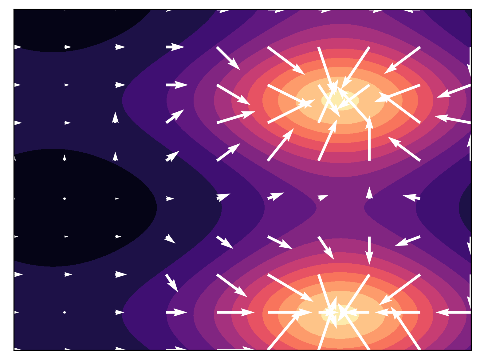
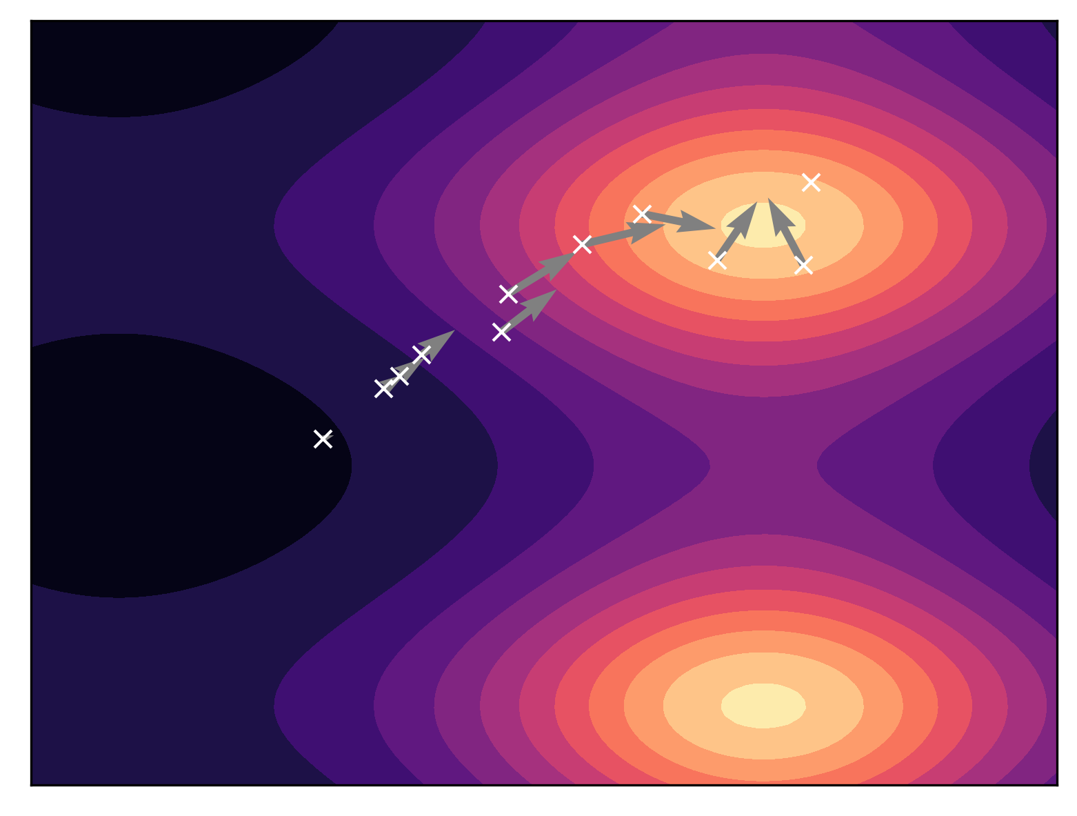
That is great! However, there is one big issue, namely, we do not know the real distribution $p_{real}(\mathbf{x})$. We are back to square one and we can use GANs, VAEs, normalizing flows, etc. for finding a model $p_{\theta}(\mathbf{x})$. Or do we? Let us have another look at (\ref{eq:sgld}). We do not require to know $p_{real}(\mathbf{x})$ but the gradient of the logarithm of the real distribution, $\nabla_{\mathbf{x}} \ln p_{real}(\mathbf{x})$. This quantity is known as the score function, $s(\mathbf{x}) \stackrel{df}{=} \nabla_{\mathbf{x}} \ln p_{real}(\mathbf{x})$. Having $s(\mathbf{x})$ allows us to run SGLD to find new points that, eventually, follow the real distribution. An example of the score function for a multimodal distribution is presented in Figure 2. The score function is represented as vectors over a grid (Figure 2 left). As we can see, the score function indicates moving towards the modes and, thus, it steers Langevine dynamics (Figure 2 right).

Figure 2. (left) An illustration of the score function $s(\mathbf{x})$ plotted as vectors (white arrows) on a regular grid for a multimodal distribution (dark colors correspond to low probability, bright colors depict high probability). (right) A trajectory after applying the SGLD (consecutive points are represented by white crosses, and their scores are denoted by gray arrows).

As a result, instead of fitting a model to the data distribution, we can fit a model to the score function. Keep in mind that the score function is a gradient, thus, it returns an object of the same shape as $\mathbf{x}$ that could be represented as a vector. Therefore, we can find the best model of the score function by optimizing the following regression problem (Hyvärinen & Dayan, 2005; Hyvärinen, 2007):

\begin{equation}\label{eq:score_matching}\tag{3} \mathcal{J}(\theta) = \frac{1}{2} \int \| s_{\theta}(\mathbf{x}) - \nabla_{\mathbf{x}} \ln p_{data}(\mathbf{x}) \|^{2}\ p_{data}(\mathbf{x})\ \mathrm{d} \mathbf{x} . \end{equation}

This integral is not anything special because it is the mean squared error loss, a typical loss used for regression.

The arising problem with (\ref{eq:score_matching}) is that it is not differentiable since $p_{data}(\mathbf{x}) = \frac{1}{N} \sum_{n=1}^{N} \delta(\mathbf{x} - \mathbf{x}_n)$, where $\delta(\cdot)$ is Dirac's delta. Since Dirac's delta is a non-differentiable function of $\mathbf{x}$, we cannot solve (\ref{eq:score_matching}) using autograd. There is a solution, though, by adding some small Gaussian noise with variance $\sigma^2$ to data, i.e., $\tilde{\mathbf{x}}_n = \mathbf{x}_n + \sigma\cdot \epsilon$, where $\epsilon \sim \mathcal{N}(0, \mathbf{I})$. The resulting distribution is Gaussian, $\mathcal{N}(\tilde{\mathbf{x}}_n | \mathbf{x}_n, \sigma^{2})$. In other words, we can turn $p_{data}(\mathbf{x})$ into a a mixture of Gaussians with data as means and some small variance $\sigma^2$, namely:

\begin{equation} q_{data}(\tilde{\mathbf{x}}_n) = \frac{1}{N} \sum_{n=1}^{N} \mathcal{N}(\tilde{\mathbf{x}}_n| \mathbf{x}_{n}, \sigma^2) . \end{equation}

Eventually, instead of using the non-differentiable objective in (\ref{eq:score_matching}), we can formulate a differentiable objective by replacing $p_{data}(\mathbf{x}_n)$ with $q_{data}(\tilde{\mathbf{x}}_n)$ in (\ref{eq:score_matching}) (Hyvärinen & Dayan, 2005; Hyvärinen, 2007; Vincent 2011):

\begin{equation}\label{eq:differentiable_score_matching}\tag{4} \mathcal{L}(\theta) = \frac{1}{2N} \sum_{n=1}^{N} \int \| s_{\theta}(\tilde{\mathbf{x}}) - \nabla_{\tilde{\mathbf{x}}} \ln \mathcal{N}(\tilde{\mathbf{x}}| \mathbf{x}_{n}, \sigma^2) \|^{2}\ \mathcal{N}(\tilde{\mathbf{x}}_n| \mathbf{x}_{n}, \sigma^2)\ \mathrm{d} \tilde{\mathbf{x}} . \end{equation}

One may say that there is still a problem because we have a gradient to calculate. However, we know the closed form of the score function for the Gaussian distribution:

\begin{align} \nabla_{\tilde{\mathbf{x}}} \ln \mathcal{N}(\tilde{\mathbf{x}}_n| \mathbf{x}_{n}, \sigma^2) &= \nabla_{\tilde{\mathbf{x}}} \left(- \ln(2\pi\sigma^D) - \frac{1}{2\sigma^2} (\tilde{\mathbf{x}}_n - \mathbf{x}_{n})^2 \right) \\ &= - \nabla_{\tilde{\mathbf{x}}} \frac{1}{2\sigma^2} (\tilde{\mathbf{x}}_n - \mathbf{x}_{n})^2 \\ &= - \frac{1}{\sigma^2} (\tilde{\mathbf{x}}_n - \mathbf{x}_{n}) \\ &= - \frac{1}{\sigma^2} (\mathbf{x}_n + \sigma\cdot \epsilon - \mathbf{x}_{n}) \\ &= - \frac{1}{\sigma} \epsilon , \end{align}

where in the fourth equation we used the definition of $\tilde{\mathbf{x}}$, $\tilde{\mathbf{x}}_n = \mathbf{x}_n + \sigma\cdot \epsilon$. Thus the score is the following:

\begin{equation}\label{eq:score_gaussian}\tag{5} \nabla_{\tilde{\mathbf{x}}} \ln \mathcal{N}(\tilde{\mathbf{x}}_n| \mathbf{x}_{n}, \sigma^2) = - \frac{1}{\sigma} \epsilon, \end{equation}

and by plugging (\ref{eq:score_gaussian}) in (\ref{eq:differentiable_score_matching}), we get the differentiable objective in the final form:

\begin{align} \mathcal{L}(\theta) &= \frac{1}{2N} \sum_{n=1}^{N} \int \| s_{\theta}(\tilde{\mathbf{x}}) + \frac{1}{\sigma} \epsilon \|^{2}\ \mathcal{N}(\epsilon | 0, \sigma^{2} \mathbf{I})\ \mathrm{d} \epsilon \\ &= \frac{1}{2N} \sum_{n=1}^{N} \mathbb{E}_{\mathcal{N}(\epsilon | 0,\mathbf{I})} \left[ \| s_{\theta}(\tilde{\mathbf{x}}) + \frac{1}{\sigma} \epsilon \|^{2} \right] \\ &= \frac{1}{N} \sum_{n=1}^{N} \mathbb{E}_{\mathcal{N}(\epsilon | 0,\mathbf{I})} \left[ \frac{1}{2\sigma} \| \epsilon - \tilde{s}_{\theta}(\tilde{\mathbf{x}}) \|^{2} \right] \label{eq:gaussian_differentiable_score_matching}\tag{6} \end{align}

where in the last line we modified the score model to be of the following form: $\tilde{s}_{\theta}(\mathbf{x}) = - \sigma s_{\theta}(\tilde{\mathbf{x}})$, and we used the property of $\sigma$ being positive (remember, it is the standard deviation that is always positive!). Of course, while implementing, we can parameterize $\tilde{s}_{\theta}(\tilde{\mathbf{x}})$ using a neural network directly, we do not have to parameterize $s_{\theta}(\mathbf{x})$ first and then rescale it, there is no need for that. We just need to be aware of all the steps here. Learning the score model $\tilde{s}_{\theta}(\tilde{\mathbf{x}})$ by optimizing the objective in (\ref{eq:gaussian_differentiable_score_matching}) is called (denoising) score matching ((Hyvärinen & Dayan, 2005; Hyvärinen, 2007; Song & Ermon, 2019).

Score matching allows us to learn a generative model in a completely different manner. Instead of matching distributions, we can perform matching scores by solving a regression problem. This is a new perspective on training generative models, but keep in mind that, eventually, this approach is used to generate data from noise by applying Langevine dynamics. Below, we gather practical information about score matching.

Score matching: Training. We can learn the score model by repeating the following steps:

1. Pick a data point $\mathbf{x}$.
2. Sample $\epsilon$ from $\mathcal{N}(\epsilon | 0, \mathbf{I})$.
3. Calculate the noisy version of data, $\tilde{\mathbf{x}} = \mathbf{x} + \sigma \cdot \epsilon$.
4. Calculate the score, $\tilde{s}_{\theta}(\tilde{\mathbf{x}})$.
5. Calculate gradient with respect to $\theta$ of the score matching objective, i.e., $\Delta \theta = \nabla_{\theta} \frac{1}{2\sigma} \| \epsilon - \tilde{s}_{\theta}(\tilde{\mathbf{x}}) \|^{2}$. We accomplish that by applying automatic differentiation.
6. Update the score model: $\theta := \theta - \Delta \theta$. Go to 1 until STOP.

In practice, we use mini-batches, but the whole procedure remains the same.

Score matching: Generation. Once we learn the score model, we can use it for sampling using Langevine dynamics. The generative procedure is the following:

1. Sample a point $\mathbf{x}_0$ at random (e.g., using a uniform distribution).
2. Run Langevine dynamics for $T$ steps, where $\Delta = \frac{1}{T}$: \begin{equation}\label{eq:score_matching_generation}\tag{7} \mathbf{x}_{t + \Delta} = \mathbf{x}_{t} + \alpha\ \tilde{s}_{\theta}(\mathbf{x}_{t}) + \eta \cdot \epsilon , \end{equation}
3. Return the final point $\mathbf{x}_1$.

The final point should follow the data distribution. Note that to keep the formulation of Langevin dynamics unchanged, we used $s_{\theta}(\mathbf{x}_{t})$ instead $\tilde{s}_{\theta}(\mathbf{x}_{t})$. There is no problem though because we know the relation $\tilde{s}_{\theta}(\mathbf{x}_{t}) = - \sigma s_{\theta}(\mathbf{x}_{t})$, thus, $s_{\theta}(\mathbf{x}_{t}) = - \frac{1}{\sigma} \tilde{s}_{\theta}(\mathbf{x}_{t})$

Score matching and Diffusion-based models. I know you, my curious reader, and I can bet you have noticed something. If we look at the objective for diffusion-based moedls in (1) and the score models in (6), we can clearly see they are almost identical (especially, if we set $\gamma_t = \frac{1}{\sigma}$)! In fact, we can turn score matching into (almost) diffusion-based approach. For this, we need three things:

1. We introduce a schedule for variances $\sigma_t^2$, for $t \in \mathcal{T} = \{t: t \text{ goes from } 0 \text{ to } 1 \text{ with the increment } \Delta = \frac{1}{T}\}$.
2. We modify the score model to be "aware" of this schedule, namely, $\tilde{s}_{\theta}(\mathbf{x}, \sigma_t^2)$.
3. We modify the objective to be "aware" of this schedule: \begin{equation} \mathcal{L}(\theta) = \frac{1}{2N} \sum_{n=1}^{N} \sum_{t \in \mathcal{T}} \lambda_t \mathbb{E}_{\mathcal{N}(\epsilon | 0,\mathbf{I})} \left[ \frac{1}{\sigma} \| \epsilon - \tilde{s}_{\theta}(\tilde{\mathbf{x}}, \sigma_t^{2}) \|^{2} \right] , \label{eq:schedule_score_matching}\tag{8} \end{equation} where $\lambda_t$ are weighting coefficients, e.g., $\lambda_t = \sigma_t^{2}$.

Sampling for such a model requires some changes. For instance, annealed Langevin dynamics could be used, see Algorithm 1 in (Song & Ermon, 2019). Eventually, we end up with a sampling procedure that is very similar to diffusion-based models. The differences lie in the sampling scheme that runs multiple steps of Langevine dynamics per each $\sigma_t^{2}$ while diffusion-based models do a single step per one "denoising".

Coding score matching

We outlined how to implement training and sampling (generation) using score matching. The code is pretty straightforward. The only "trick" is to transform data to be in $[-1, 1]$. In the code below, we make only one difference compared to our analysis above, namely, we use $\frac{1}{2\sigma} \| \epsilon + \tilde{s}_{\theta}(\tilde{\mathbf{x}}) \|^{2}$ such that Langevine dynamics is in its standard form: $\mathbf{x}_{t + \Delta} = \mathbf{x}_{t} + \alpha\ \tilde{s}_{\theta}(\mathbf{x}_{t}) + \eta \cdot \epsilon$.

The full code (with auxiliary functions) that you can play with is available here: link.

class ScoreMatching(nn.Module):
    def __init__(self, snet, alpha, sigma, eta, D, T):
        super(ScoreMatching, self).__init__()

        print('Score Matching by JT.')

        self.snet = snet
        
        # other hyperparams
        self.D = D
                
        self.sigma = sigma
        
        self.T = T
        
        self.alpha = alpha
        
        self.eta = eta
    
    def sample_base(self, x_1):
        # Uniform over [-1, 1]**D
        return 2. * torch.rand_like(x_1) - 1.
    
    def langevine_dynamics(self, x):
        for t in range(self.T):
            x = x + self.alpha * self.snet(x) + self.eta * torch.randn_like(x)
        return x

    def forward(self, x, reduction='mean'):
        # =====Score Matching
        # sample noise
        epsilon = torch.randn_like(x)
        
        # =====
        # calculate the noisy data
        tilde_x = x + self.sigma * epsilon

        # =====
        # calculate the score model
        s = self.snet(tilde_x)
        
        # =====LOSS: the Score Matching Loss
        SM_loss = (1. / (2. * self.sigma)) * ((s + epsilon)**2.).sum(-1) # in order to keep the Langevine dynamics unchanged, we do not use \tilde{s} = -sigma * s but we use \tilde{s} = sigma * s
        
        # Final LOSS
        if reduction == 'sum':
            loss = SM_loss.sum()
        else:
            loss = SM_loss.mean()

        return loss

    def sample(self,  batch_size=64):
        # sample x_0
        x = self.sample_base(torch.empty(batch_size, self.D))
        
        # run langevine dynamics
        x = self.langevine_dynamics(x)
        
        x = torch.tanh(x)
        return x

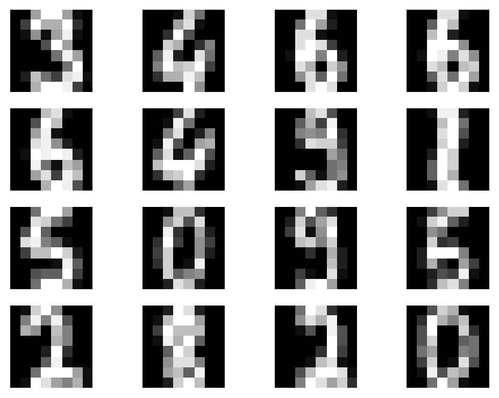
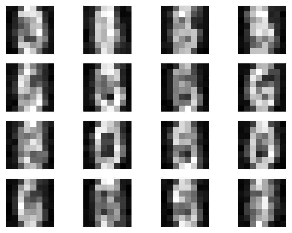
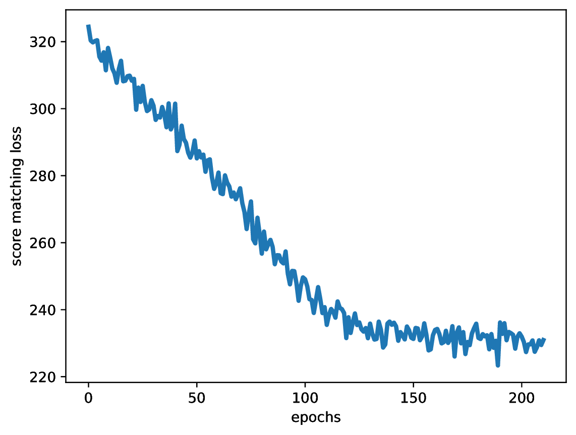
After running the code with an MLP-based scoring model, and the following values of the hyperparameters $\alpha = 0.1$, $\sigma=0.1$, $\eta=0.05$ and $T=100$, we can expect results like in Figure 3.

A

B

C

Figure 3. A. A sample of real images. B. A sample of generated images. C. An example of the score matching loss caluclated on the validation set.

What we can do with score matching?

Improving score matching. As we can see, we can get some (quite reasonable) generations using an extremely simplistic code. However, there are some issues with score matching as indicated in the original paper (Song & Ermon, 2019):

• First and foremost, low density regions (i.e., regions with little to none data) can cause difficulties in score estimation. Take a look at Figure 2. left again, and look closer at the real score in the dark areas. In these regions there is very unlikely to see any datapoint. As a result, we can very badly estimate the score function.
• Second issue follows from the first one, namely, for a badly trained score model, Langevin dynamics could result in bad samples. To some degree, we can see that in our example in Figure 3.B.
• Third, if modes of a real data distribution are far away, Langevine dynamics would require multiple steps to reach them. This problem is known as slow mixing.

To overcome these issues, we can use the following methods:

• Instead of using a single variance, we can choose a sequence of variances and the annealed Langevine dynamics method, as discussed earlier. For details, we recommend (Song & Ermon, 2019) and a follow-up with other useful tricks (Song & Ermon, 2020).
• A better score model, especially for high-dimensional cases, could be trained by following sliced score matching (Song et al., 2020). The idea is similar to Sliced Wasserstein distance (Rabin et al., 2012) in which the score function and the score model are projected onto some random direction. Then, the new sliced score matching objective is easier to calculate (it requires only vector multiplication). This new objective is closely related to Hutchinson’s trace estimator.

Other extensions. Score matching is a general framework that could be further extended. Here are some examples:

• Score matching is a suitable approach for energy-based models. This idea was used for learning Boltzmann Machines (Marlin et al. 2010; Swersky et al., 2011), and other energy-based models (Li et al., 2023).
• The idea of matching scores of distributions over random variables could be utilized in learning distributions over discrete random variables (Meng et al., 2022). For this, we need to use a different definition of scores, appropriate for probability mass functions.
• Score matching could be used beyond images. In (Luo & Hu, 2021), the authors proposed a method for modeling point clouds. Their approach utilized a specific kind of a score model that is feasible for processing cloud of points.

References

(Ho et al., 2020) Ho, J., Jain, A. and Abbeel, P., 2020. Denoising diffusion probabilistic models. Advances in neural information processing systems, 33, pp.6840-6851.

(Hyvärinen & Dayan, 2005) Hyvärinen, A. and Dayan, P., 2005. Estimation of non-normalized statistical models by score matching. Journal of Machine Learning Research, 6(4).

(Hyvärinen, 2007) Hyvärinen, A., 2007. Some extensions of score matching. Computational statistics & data analysis, 51(5), pp.2499-2512.

(Kingma et al., 2021) Kingma, D., Salimans, T., Poole, B. and Ho, J., 2021. Variational diffusion models. Advances in neural information processing systems, 34, pp.21696-21707.

(Kingma & Gao, 2023) Kingma, D.P. and Gao, R., 2023, November. Understanding diffusion objectives as the ELBO with simple data augmentation. In Thirty-seventh Conference on Neural Information Processing Systems.

(Li et al., 2023) Li, Z., Chen, Y. and Sommer, F.T., 2023. Learning Energy-Based Models in High-Dimensional Spaces with Multiscale Denoising-Score Matching. Entropy, 25(10), p.1367.

(Luo & Hu, 2021) Luo, S. and Hu, W., 2021. Score-based point cloud denoising. In Proceedings of the IEEE/CVF International Conference on Computer Vision (pp. 4583-4592).

(Marlin et al. 2010) Marlin, B., Swersky, K., Chen, B. and Freitas, N., 2010, March. Inductive principles for restricted Boltzmann machine learning. In Proceedings of the thirteenth international conference on artificial intelligence and statistics (pp. 509-516). JMLR Workshop and Conference Proceedings.

(Meng et al., 2022) Meng, C., Choi, K., Song, J. and Ermon, S., 2022. Concrete score matching: Generalized score matching for discrete data. Advances in Neural Information Processing Systems, 35, pp.34532-34545.

(Rabin et al., 2012) Rabin, J., Peyré, G., Delon, J. and Bernot, M., 2012. Wasserstein barycenter and its application to texture mixing. In Scale Space and Variational Methods in Computer Vision: Third International Conference, SSVM 2011, Ein-Gedi, Israel, May 29–June 2, 2011, Revised Selected Papers 3 (pp. 435-446). Springer Berlin Heidelberg.

(Sohl-Dickstein et al., 2015) Sohl-Dickstein, J., Weiss, E., Maheswaranathan, N. and Ganguli, S., 2015, June. Deep unsupervised learning using nonequilibrium thermodynamics. In International conference on machine learning (pp. 2256-2265). PMLR.

(Song & Ermon, 2019) Song, Y. and Ermon, S., 2019. Generative modeling by estimating gradients of the data distribution. Advances in neural information processing systems, 32.

(Song & Ermon, 2020) Song, Y. and Ermon, S., 2020. Improved techniques for training score-based generative models. Advances in neural information processing systems, 33, pp.12438-12448.

(Song et al., 2020) Song, Y., Garg, S., Shi, J. and Ermon, S., 2020, August. Sliced score matching: A scalable approach to density and score estimation. In Uncertainty in Artificial Intelligence (pp. 574-584). PMLR.

(Song et al., 2021) Song, Y., Durkan, C., Murray, I. and Ermon, S., 2021. Maximum likelihood training of score-based diffusion models. Advances in Neural Information Processing Systems, 34, pp.1415-1428.

(Swersky et al., 2011) Swersky, K., Ranzato, M.A., Buchman, D., Freitas, N.D. and Marlin, B.M., 2011. On autoencoders and score matching for energy based models. In Proceedings of the 28th international conference on machine learning (ICML-11) (pp. 1201-1208).

(Vincent 2011) Vincent, P., 2011. A connection between score matching and denoising autoencoders. Neural computation, 23(7), pp.1661-1674.

(Welling & Teh, 2011) Welling, M. and Teh, Y.W., 2011. Bayesian learning via stochastic gradient Langevin dynamics. In Proceedings of the 28th international conference on machine learning (ICML-11) (pp. 681-688).