Flow Matching: Matching flows instead of scores
A different perspective on generative models with ODEs: Continuous Normalizing Flows (CNFs)
About ODEs, again. Previously, we discussed how generative models could be defined through Stochastic Differential Equations (SDEs) or, equivalently, corresponding Probability Flow Ordinary Differential Equations (PF-ODEs). We showed that by solving SDEs/ODEs using a numerical solver like backward Euler's method, we obtain an iterative generative procedure of turning noise into data. However, there is a question whether we need to first formulate an SDE and its PF-ODE equivalent, or maybe we can take any ODE to define a generative model. I know you, my curious reader, and I feel you! We use SDEs because we know they are trained by score matching. If we take any ODE, how could we learn such generative models?
Let us be more concrete here. We recall the definition of an ODE:
\begin{equation} \frac{\mathrm{d} \mathbf{x}_t}{\mathrm{d} t} = v(\mathbf{x}_{t}, t) , \end{equation}where the vector field, $v(\mathbf{x}_{t}, t)$, defines the dynamics. Parameterizing the vector field with a neural network with weights $\theta$, $v_{\theta}(\mathbf{x}_{t}, t)$, leads to a so-called neural ODE (Chen et al., 2018). If we denote by $\mathbf{x}_{0}$ the initial condition for this neural ODE, e.g., noise, then by solving it, i.e., integrating over time $t$, we get the output (e.g., data):
\begin{equation} \mathbf{x}_{1} = \int_{0}^{1} v_{\theta}(\mathbf{x}_{t}, t) \mathrm{d} t . \end{equation}So far so good, but there is (almost) nothing new compared to score-based generative models where we match scores instead of distributions (i.e., an empirical distribution to a model). Could we formulate a likelihood-based training? The short answer is: Yes. Is it easy? Again, the short answer: No. But let us look into both answers more in details.
From the continuity equation (conservation of mass) to the instantaneous change of variables. Again, sampling from an ODE, namely, integrating from $t=0$ to $t=1$ is not difficult once we have a model of the vector field. We can use Euler's method for that (or any other numerical solver). However, obtaining the model is problematic if we prefer fitting a data distribution to a distribution induced by $v_{\theta}(x, t)$. After all, starting with a known distribution $\mathbf{x}_{0} \sim \pi(\mathbf{x})$ like standard Gaussian, and then solving the ODE yields another distribution! We can express this induced distribution analytically using the continuity equation. Here comes some math (and even physics!), so buckle up and let us dive in.
Imagine for a second that probability is a mass (I always think of clay, but it could be water, if you prefer), something we can touch with our fingers. Now let us visualize a pipe of the same cross-section volume across its length in which our mass (e.g., water) flows. At each moment of time, we have some flux of this mass, $f_t$, i.e., our (probability) mass is moved according to the vector field (or velocity), $f_t(\mathbf{x}_t) = p_t(\mathbf{x}_t) v(\mathbf{x}_{t}, t)$. Since we talk about probability mass (or water flowing through the pipe of the same volume of cross-sections everywhere), the mass is conserved, i.e., no new mass (water) (dis)appears (no leaking or pouring in). Mathematically, it means that the change of the mass $\frac{\partial p_t(\mathbf{x}_t)}{\partial t}$ plus the change of the flux volume in all directions (a.k.a. the divergence of the flux) is constant (i.e., the mass is conserved):
where $\mathrm{div} \left(\cdot\right)$ is the divergence defined as follows: $\mathrm{div} \left( V(x_1, \ldots, x_D) \right) = \sum_{d=1}^{D} \frac{\partial V_d(x_1, \ldots, x_D)}{\partial x_d}$, i.e., the sum of first derivatives of $V$ over all variables separately.
As a side note, it is good to notice that the trace of the Jacobian matrix is the divergence of the vector field! For a two-dimensional space and a vector field $V(x_1, x_2)$, $\mathrm{div} \left( V(x_1, x_2) \right) = \frac{\partial V_1(x_1, x_2)}{\partial x_1} + \frac{\partial V_2(x_1, x_2)}{\partial x_2} = \mathrm{Tr}\left( \frac{\partial V_i(x_1, x_2)}{\partial x_i} \right)$, where $\frac{\partial V_i(x_1, x_2)}{\partial x_i} = \begin{bmatrix} \frac{\partial V_{1}}{\partial x_1} & \frac{\partial V_{1}}{\partial x_2} \\ \frac{\partial V_{2}}{\partial x_1} & \frac{\partial V_{2}}{\partial x_2} \end{bmatrix}$ is the Jacobian matrix, and $\mathrm{Tr}(\mathbf{A}) = \sum_{i} \mathbf{A}_{ii}$ is the trace of a matrix $\mathbf{A}$.
It turns out that applying identities of vector calculus and the properties of the divergence allows us to write the continuity equation using the logarithm of the probability distribution (a.k.a. the instantaneous change of variables (Chen et al., 2018)):
\begin{equation} \frac{\mathrm{d} \ln p(\mathbf{x}_t)}{\mathrm{d} t} + \mathrm{Tr}\left( \frac{\partial v(\mathbf{x}_{t}, t)}{\partial \mathbf{x}_t} \right) = 0 . \end{equation}I know you, my curious reader, you dislike being told about something without a proof. It is a side note, so if you do not have time for it, just skip it. But I find this pretty cool and it will be also helpful in our further discussion. OK, so what do we need? First, a general property: $\frac{\partial \ln p_{t}}{\partial t} = \frac{1}{p_{t}} \frac{\partial p_{t}}{\partial t}$, or: $p_{t} \frac{\partial \ln p_{t}}{\partial t} = \frac{\partial p_{t}}{\partial t}$. Second, we have: $\mathrm{div}(p_t v) = \langle \nabla_{\mathbf{x}} p_t, v \rangle + p_t \mathrm{div}(v)$, hence, $\frac{\mathrm{div}(p_t v)}{p_t} = \langle \nabla_{\mathbf{x}} \ln p_t, v \rangle + \mathrm{div}(v)$. Third, we saw already that the divergence of the vector field equals its trace. Now, we can plug these three facts to the continuity equation: \begin{align} \frac{\partial p_t(\mathbf{x}_t)}{\partial t} + \mathrm{div} \left( p_t(\mathbf{x}_t) v(\mathbf{x}_{t}, t) \right) &= 0\\ \frac{1}{p_t(\mathbf{x}_t)} \frac{\partial p_t(\mathbf{x}_t)}{\partial t} + \frac{1}{p_t(\mathbf{x}_t)} \mathrm{div} \left( p_t(\mathbf{x}_t) v(\mathbf{x}_{t}, t) \right) &= 0\\ \frac{\partial \ln p_t(\mathbf{x}_t)}{\partial t} + \langle \nabla_{\mathbf{x}} \ln p_t, v \rangle + \mathrm{div} \left( v(\mathbf{x}_{t}, t) \right) &= 0 \\ \langle \nabla_{\mathbf{x}} \ln p_t, v \rangle = -\frac{\partial \ln p_t(\mathbf{x}_t)}{\partial t} - \mathrm{div} \left( v(\mathbf{x}_{t}, t) \right) \end{align}
Next, calculating the total derivative of $\ln p_t(\mathbf{x}_t)$ and plugging in the above equation for $\langle \nabla_{\mathbf{x}} \ln p_t, v \rangle $ , we get the following (Ben-Hamu et al., 2022):
\begin{align} \frac{\mathrm{d} \ln p(\mathbf{x}_t)}{\mathrm{d} t} &= \langle \frac{\partial \ln p(\mathbf{x}_t)}{\partial t}, \frac{\partial t}{\partial t} \rangle + \langle \nabla_{\mathbf{x}} \ln p(\mathbf{x}_t), \frac{\partial \mathbf{x}_t}{\partial t} \rangle \\ &= \frac{\partial \ln p(\mathbf{x}_t)}{\partial t} + \langle \nabla_{\mathbf{x}} \ln p(\mathbf{x}_t), \frac{\partial \mathbf{x}_t}{\partial t} \rangle \\ &= \frac{\partial \ln p(\mathbf{x}_t)}{\partial t} + \langle \nabla_{\mathbf{x}} \ln p(\mathbf{x}_t), v(\mathbf{x}_t , t) \rangle \\ &= \frac{\partial \ln p(\mathbf{x}_t)}{\partial t} - \frac{\partial \ln p_t(\mathbf{x}_t)}{\partial t} - \mathrm{div} \left( v(\mathbf{x}_{t}, t) \right) \\ &= - \mathrm{div} \left( v(\mathbf{x}_{t}, t) \right) \\ &= - \mathrm{Tr}\left( \frac{\partial v(\mathbf{x}_{t}, t)}{\partial \mathbf{x}_t} \right) \end{align}
Then, by integrating across time, we can compute the total change in log-density as follows:
\begin{align} \int_{0}^{1} \left( \frac{\mathrm{d} \ln p(\mathbf{x}_t)}{\mathrm{d} t} + \mathrm{Tr}\left( \frac{\partial v(\mathbf{x}_{t}, t)}{\partial \mathbf{x}_t} \right) \right) \mathrm{d}t &= 0 \\ \ln p(\mathbf{x}_1) - \ln \pi(\mathbf{x}_0) + \int_{0}^{1} \mathrm{Tr}\left( \frac{\partial v(\mathbf{x}_{t}, t)}{\partial \mathbf{x}_t} \right) \mathrm{d}t &= 0 \\ \ln p(\mathbf{x}_1) &= \ln \pi(\mathbf{x}_0) - \int_0^1 \mathrm{Tr}\left( \frac{\partial v(\mathbf{x}_{t}, t)}{\partial \mathbf{x}_t} \right) \mathrm{d} t . \end{align}Why do we bother to calculate everything as log-probabilities? Because the last line is a continuous version of the change of variables used for normalizing flows! Here, we have the integral over time of the trace of the Jacobian matrix instead of the sum of the log-determinants of the Jacobian matrix. Therefore, training neural ODEs is similar to training normalizing flows but with continuous time. As a result, neural ODEs in this context are refered to as continuous normalizing flows (CNFs).
Calculating the log-likelihood for CNFs. However, unlike in discrete time normalizing flows, we do not require invertibility of $v$, thus, for given datapoint $\mathbf{x}_1$, typically, we cannot simply invert the transformation to obtain $\mathbf{x}_0$. However, under pretty mild conditions (namely, $v$ and its first derivative are Lipschitz continuous, e.g., for a neural net with Lipschitz continuous activation functions like SELU or SiLU, among others), we can uniquely solve the following problem (Grathwohl et al., 2018):
with the following initial conditions:
\begin{equation} \begin{bmatrix} \mathbf{x}_1 \\ \ln p_1(\mathbf{x}_{data}) - \ln p_{1}(\mathbf{x}_1) \end{bmatrix} = \begin{bmatrix} \mathbf{x}_{data} \\ 0 , \end{bmatrix} \end{equation}in which $\mathbf{x}_1$ is a datapoint $\mathbf{x}_{data}$, and the difference in log-probability is zero. Note that we solve the problem in the reverse order, namely, from data $\mathbf{x}_1$ to noise $\mathbf{x}_0$.
To sum up, we need to do the following:
- Take a datapoint $\mathbf{x}_1 = \mathbf{x}_{data}$.
- Solve the problem in (\ref{eq:cnf_likelihood}) by applying a solver to find $\mathbf{x}_0$ and keeping track of traces over time.
- Calculate the log-likelihood by adding $\ln \pi(\mathbf{x}_0)$ to the sum of negative traces $- \int_0^1 \mathrm{Tr}\left( \frac{\partial v_{\theta}(\mathbf{x}_{t}, t)}{\partial \mathbf{x}_t} \right) \mathrm{d} t$.
Now we can backpropagate through a solver and viola! Or really? What about complexity of this whole procedure? At the first glance, it seems very expensive...
Hutchinson's trace estimator. If you remember correctly, my curious reader, the problem with normalizing flows was about calculating the log-determinant of the Jacobian matrix of size $D \times D$, which in general case costs $\mathcal{O}(D^3)$. Computing the trace requires $\mathcal{O}(D^2)$ since we need the sum of the diagonal, but each entry in the diagonal requires a separate forward propagation, thus, the quadratic complexity. It is better than in the discrete case, but there is another caveat: We need to backpropagate through a numerical solver! No free lunch, I am afraid... (Chen et al., 2018) proposed to use the adjoint sensitivity method, which could be seen as a version of backpropagation with the continuous time. Then, the neural ODE is trained by maximizing the log-likelihood $\ln p(\mathbf{x}_1)$. However, it requires running the numerical method to solve the ODE and then backpropagating through it for each new datapoint. This is a very costly operation!
As a result, we need to look for improvements to cut costs everywhere we can. One trick we can apply is about caclulating the trace. By utilizing Hutchinson's trace estimator (Grathwohl et al., 2018), the quadratic complexity is decreased to $\mathcal{O}(D)$, and it is relatively easy to calculate for any square matrix $\mathbf{A}$, namely:
where $\epsilon$ follows a distribution with zero mean and a unit variance, e.g., $\epsilon \sim \mathcal{N}(0, \mathbf{I})$. For a specific $\epsilon$, the product of $\mathbf{A} \epsilon$ could be calculated in a single forward pass and it is "backpropagatable", therefore, we can estimate the trace by taking $M$ Monte Carlo samples:
\begin{equation} \mathrm{Tr}(\mathbf{A}) \approx \frac{1}{M} \sum_{m=1}^{M} \epsilon_m^{\top} \mathbf{A} \epsilon_m . \end{equation}
In practice, we take $M=1$, namely, a single sample of $\epsilon$ for every newly coming datapoint. This is a noisy estimate, obviously, however, it is unbiased. As a result, during training with a stochastic gradient-based method, it does not matter too much.
Eventually, we obtain a procedure that is $\mathcal{O}(D)$ plus the cost of running the adjoint sensitivity method (a specific numerical solver). Overall, not bad, but far from fantastic. We do not even provide a code here, because scaling up CNFs is a known problem. Is there any alternative then? Can we do better? Of course, my curious reader, of course we can!
Going with the flow: Flow Matching
Let us take another look at the ODE we introduced earlier:
\begin{equation} \frac{\mathrm{d} \mathbf{x}_t}{\mathrm{d} t} = v(\mathbf{x}_{t}, t) . \end{equation}Additionally to this ODE, we assume a known distribution $q_{0}(\mathbf{x})$ (e.g., the standard Gaussian) and a data distribution $q_{1}(\mathbf{x})$.
NOTE: To stay consistent with the flow matching literature, we now go from noise ($t=0$) to data ($t=1$), which defines the forward dynamics and, thus, the generative process. Unlike the diffusion models (and score-based models), where the time goes in the other direction, i.e., from data to noise.
We know from our discussion on CNFs above that the distribution defined at any moment $t$ is characterized by the continuity equation. And, moreover, by applying the instantaneous change of variables, we can find a solution, i.e., a probability distribution. However, all of this sounds quite complicated and, as discussed earlier, it results in pretty computationally heavy training. What can we do then? Or, a different question is, what we could do if we knew the vector field $v(\mathbf{x}_{t}, t)$ and distributions $p_{t}(\mathbf{x})$. How could we train our model then? And what would be our model? Do you remember the score matching approach? Take a look at the denoising score matching loss again. What if we apply a similar approach here, namely, instead of looking for a distribution, we find a model of the vector field $v_{\theta}(\mathbf{x}_{t}, t)$. Similar to score matching, we solve the regression problem in the following form:
\begin{equation} \ell_{FM}(\theta) = \mathbb{E}_{t\sim U(0,1), \mathbf{x}_t \sim p_{t}(\mathbf{x})}\left[ \|v_{\theta}(\mathbf{x}_{t}, t) - v(\mathbf{x}_{t}, t) \|^2 \right] , \end{equation}
instead of looking for a distribution like in CNFs. In plain words, for any time $t$ sampled uniformly at random, we sample $\mathbf{x}_{t}$ from the distribution $p_{t}(\mathbf{x})$ (we assume we know it!) and aim at minimizing the difference between the model $v_{\theta}(\mathbf{x}_{t}, t)$ and the real vector field $v(\mathbf{x}_{t}, t)$ (we assume we know it!). We refer to this objective as flow matching (FM).
Why would this work? For a very simple reason: If $\ell_{FM}(\theta) = 0$, i.e., our model perfectly imitates the real vector field, we can transform any noise distribution to the data distribution! Why? Because the vector field pushes points towards the data distribution over time. Take a look at Figure 1 where blue arrows (the vector field) indicate how points should evolve over time from a noise distribution $q_0(\mathbf{x})$ (e.g., the standard Gaussian) to the data distribution $q_1(\mathbf{x})$ (orange half-moons in Figure 1).
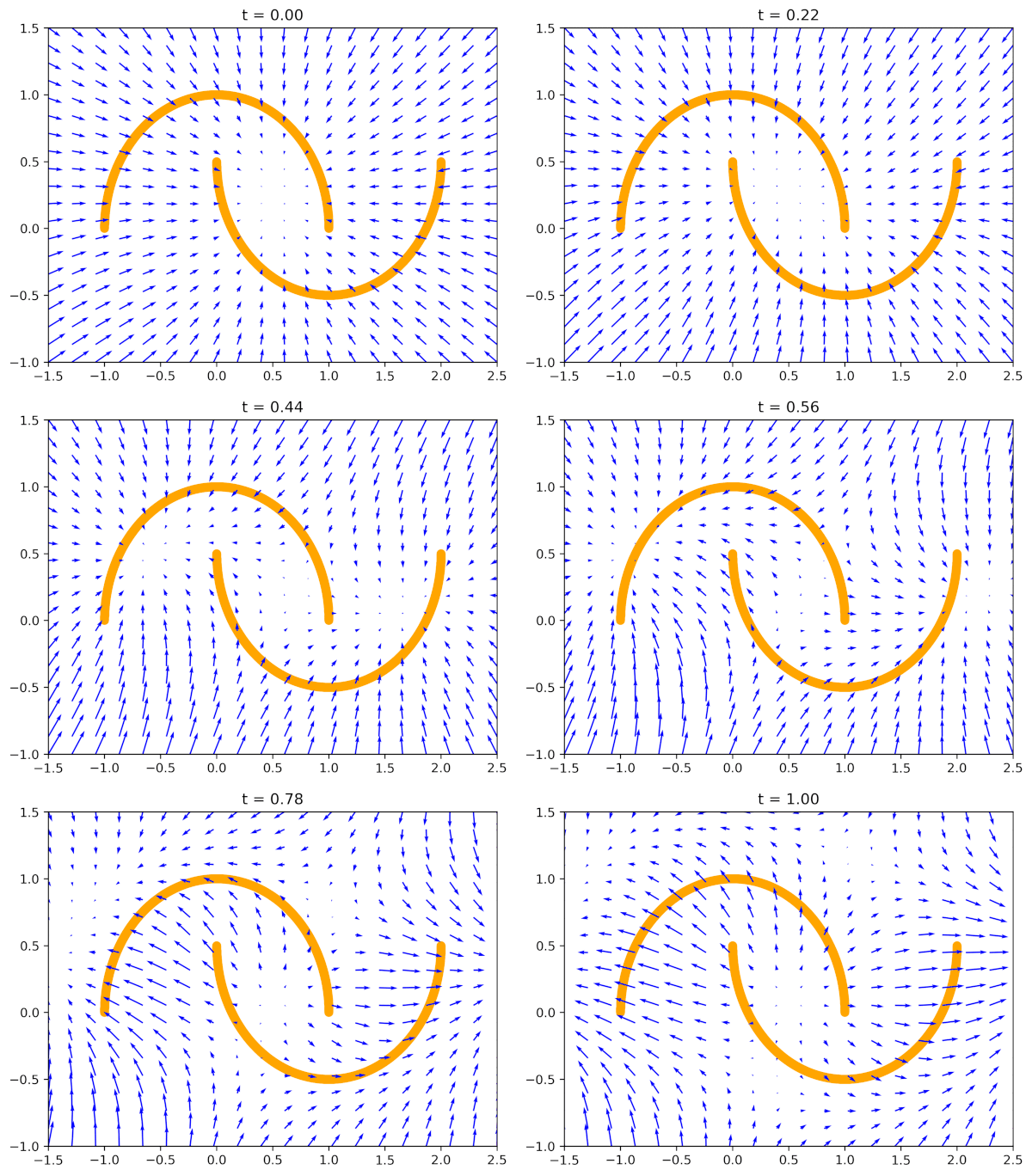
The second question is why this is so great? The answer is (again) simple: This is the regression problem, the mean squared error loss! Nothing complicated, nothing tricky, a well-behaved convex loss. One can run autograd, and use any deep learning library to implement that. Fantastic!
But... Here comes the "but": We do not know $p_{t}(\mathbf{x})$ and $v(\mathbf{x}_{t}, t)$. I know you, my curious reader, you kept it in your head throughout the whole discussion so far. You are polite, so you waited patiently. I would already say "bollocks", the assumption that we know both the vector field and the distributions $p_{t}(\mathbf{x})$ is simply bollocks. What we can do about it then, you ask? In the following, we will show how to deal with that!
Conditional Flow Matching. First, let us consider a modified problem in which we introduce additional variables $\mathbf{z}$ sampled from a given distribution $q(\mathbf{z})$. The conditional ODE takes the following form:
For now, please think of this problem as a proxy for the unconditional ODE introduced before. In general, it is typically easier to work with conditional problems as long as the conditioning information is relevant. Regarding $\mathbf{z}$, we can think of it as extra information like data $\mathbf{x}_1$, or anything else like a class label, a piece of text, an audio signal, or an additional image. Then, since we have to also sample $\mathbf{z}$'s from some distribution $q(\mathbf{z})$, the conditional flow matching (CFM) loss can be defined as follows:
\begin{equation} \ell_{CFM}(\theta) = \mathbb{E}_{t\sim U(0,1), \mathbf{x}_t \sim p_{t}(\mathbf{x} | \mathbf{z}), \mathbf{z} \sim q(\mathbf{z})}\left[ \|v_{\theta}(\mathbf{x}_{t}, t) - v(\mathbf{x}_{t}, t; \mathbf{z}) \|^2 \right] , \end{equation}
where we still use an unconditional model of the conditional vector field.
In the CFM loss, we need to define the conditional distribution at every $t$, $p_{t}(\mathbf{x} | \mathbf{z})$, and the real vector field is conditioned on $\mathbf{z}$, $v(\mathbf{x}_{t}, t; \mathbf{z})$. At first, the CFM problem does not seem to be very useful regarding the FM problem. Why would adding conditioning help to learn a model that should work for the unconditional case? As proved in (Lipman et al., 2022) and (Tong et al., 2023), both losses are equal up to a constant independent of $\theta$, and, thus, their gradients are equal!
Theorem 1 (Lipman et al., 2022) If $p_{t}(\mathbf{x}) > 0$ for all $\mathbf{x} \in \mathbb{R}^D$ amd $t \in [0, 1]$, then, up to a constant independent of $\theta$, $\ell_{FM}$ and $\ell_{CFM}$ are equal, and hence $\nabla_{\theta} \ell_{FM}(\theta) = \nabla_{\theta} \ell_{CFM}(\theta)$.
This is a marvelous result! It means that the model $v_{\theta}(\mathbf{x}, t)$ trained with the conditional version of the loss, but which is unconditional, coincides with the solution of the unconditional flow matching problem. Fantastic! One problem is gone, we can use CFM instead of FM! Alright, but now we have another problem, namely, what this conditioning $\mathbf{z}$ should be, and what is its distribution $q(\mathbf{z})$. Fortunately, there are multiple options (see, e.g., (Tong et al., 2023)), here we focus on two of those:
- In Lipman et al. CNF, $\mathbf{z}$ is a datapoint $\mathbf{x}_1$, and thus, $q(\mathbf{z}) = q_{1}(\mathbf{z})$; in other words, $q(\mathbf{z})$ is the data distribution.
- In Tong et al. CNF (a.k.a. independent CFM, iCFM), $\mathbf{z}$ is a pair of noise and data, $\mathbf{z} = (\mathbf{x}_0, \mathbf{x}_1)$, sampled independently from each other, i.e., $q_0(\mathbf{z}) = q(\mathbf{x}_{0})\ q_{1}(\mathbf{x}_{1})$.
An extension of iCFM is sampling $\mathbf{z} = (\mathbf{x}_0, \mathbf{x}_1)$ by solving the optimal transport problem. Interested readers (yes, you!) should check out (Tong et al., 2023) for further details.
Conditional probability paths. Now we know that we can consider the conditional flow matching problem as the perfect proxy to the uncoditional flow matching problem. However, the last piece of the puzzle is how to obtain conditional distributions $p_{t}(\mathbf{x} | \mathbf{z})$ a.k.a. (conditional) probability paths. We know from our discussions on CNFs that the continuity equation allows us to calculate the probability path. But for that, we need to know the vector field. It is a classical example of circular reasoning. How to avoid it?
My curious reader, so far you have learnt a lot about AI and you probably can guess already what is the simplest approach we can take here. Do I hear properly? Do you whisper Gaussians? Yes, indeed! Let us consider the form of $p_{t}(\mathbf{x} | \mathbf{z})$ first, and then, from that, we will derive the vector field $v(\mathbf{x}, t; \mathbf{z})$. This is probably a limiting factor of the whole approach, but dang, we want to calculate something, and is there a better candidate than Gaussian? Let us consider the conditional probability path of the following form:
\begin{equation} p_{t}(\mathbf{x} | \mathbf{z}) = \mathcal{N}(\mathbf{x} | \mu(\mathbf{z}, t), \sigma^2(\mathbf{z}, t) \mathbf{I}) , \end{equation}
which is a Gaussian distribution with the mean function $ \mu(\mathbf{z}, t)$ and a diagonal covariance matrix with the standard deviation function $\sigma(\mathbf{z}, t)$. In general, there is no unique ODE that generates these distributions. However, the following theorem shows that there is the unique vector field that leads to those!
Theorem 2 (Lipman et al., 2022) The unique vector field with initial conditionas $p_{0}(\mathbf{x}) = \mathcal{N}(\mu_0, \sigma_0^2 \mathbf{I})$ that generates $p_{t}(\mathbf{x} | \mathbf{z}) = \mathcal{N}(\mathbf{x} | \mu(\mathbf{z}, t), \sigma^2(\mathbf{z}, t) \mathbf{I})$ has the following form: \begin{equation} v(\mathbf{x}, t; \mathbf{z}) = \frac{\sigma^{'}(\mathbf{z}, t)}{\sigma(\mathbf{z}, t)} \left(\mathbf{x} - \mu(\mathbf{z}, t) \right) + \mu^{'}(\mathbf{z}, t), \end{equation} where $\sigma^{'}(\mathbf{z}, t)$ and $\mu^{'}(\mathbf{z}, t)$ denote the time derivates of $\sigma(\mathbf{z}, t)$ and $\mu(\mathbf{z}, t)$, respectively.
Ok, we should stop and think of it for a while, maybe read it again. You got it? Yes, this theorem gives us an incredible result! If we consider a class of conditional probability paths in the form of Gaussians, we can analytically calculate the conditional vector field as long as the means and the standard deviations are differentiable. In other words, we have a general presciption for flow matching! First, we define means and standard deviations as functions of $\mathbf{z}$ and time $t$. Second, for given forms of the means and the standard deviations, we calculate the conditional vector field. Third, we optimize the conditional flow matching loss for a given vector field model. That is all, as simple as it is. To get a better understanding how it works, we look into two specific forms of conditional flow matching, namely:
- Lipman et al. CFM (we refer to it as 'fm' later on in the code): We take $\mathbf{z} \equiv \mathbf{x}_1$ to be data sampled form the data distribution, $\mathbf{x}_1 \sim q_{1}(\mathbf{x})$. Then, we define the mean and the standard deviation functions as follows:
\begin{align} \mu(\mathbf{z}, t) &= t \mathbf{x}_1 ,\\ \sigma(\mathbf{z}, t) &= t \sigma_{const} - t + 1 , \end{align}
where $\sigma_{const} > 0$ is a smoothing constant. As a result, we obtain the following conditional probability path and the conditional vector field:
\begin{align} p_{t}(\mathbf{x} | \mathbf{z}) &= \mathcal{N}\left( \mathbf{x} | t \mathbf{x}_1, (t \sigma_{const} - t + 1)^2 \mathbf{I} \right) , \\ v(\mathbf{x}, t ; \mathbf{z}) &= \frac{ \mathbf{x}_1 - (1 - \sigma_{const}) \mathbf{x} }{ 1 - (1 - \sigma_{const}) t } . \end{align}
To obtain the analytical form of $v(\mathbf{x}, t ; \mathbf{z})$, we need to apply the theorem presented above. It turns out that we get a probability path from the standard Gaussian distribution, $p_0(\mathbf{x}) = \mathcal{N}(\mathbf{x} | 0, \mathbf{I})$, to a Gaussian distribution centered at a datapoint with standard deviation $\sigma_{const}$, $p_1(\mathbf{x}) = \mathcal{N}(\mathbf{x} | \mathbf{x}_1, \sigma_{const}^2 \mathbf{I})$ (Lipman et al., 2022).
- Tong et al. iCFM: We consider $\mathbf{z} \equiv (\mathbf{x}_0, \mathbf{x}_1)$ and $q(\mathbf{z}) = q_0(\mathbf{x}_0) q_1(\mathbf{x}_1)$. Next, we choose the following means and standard deviations:
\begin{align} \mu(\mathbf{z}, t) &= t \mathbf{x}_1 + (1 - t) \mathbf{x}_0 ,\\ \sigma(\mathbf{z}, t) &= \sigma_{const} , \end{align}
where $\sigma_{const} > 0$ is a smoothing constant. The mean function is an interpolation between noise and data since $t \in [0, 1]$. The resulting conditional probability path and the conditional vector fields are the following:
\begin{align} p_{t}(\mathbf{x} | \mathbf{z}) &= \mathcal{N}\left( \mathbf{x} | t \mathbf{x}_1 + (1 - t) \mathbf{x}_0, \sigma_{const}^2 \mathbf{I} \right) , \\ v(\mathbf{x}, t ; \mathbf{z}) &= \mathbf{x}_1 - \mathbf{x}_0 . \end{align}
Interestingly, the vector field results in a difference between a data point and a sampled noise. This comes from the fact that we assume fixed standard deviation in the probability path and, after applying Theorem 2, we end up with the derivate of the mean function only. (Tong et al., 2023) showed (see Proposition 3.3 therein) that the boundry distributions are $p_0(\mathbf{x}) = q_0(\mathbf{x}) * \mathcal{N}(\mathbf{x} | 0, \sigma_{const}^2 \mathbf{I})$ and $p_1(\mathbf{x}) = q_1(\mathbf{x}) * \mathcal{N}(\mathbf{x} | 0, \sigma_{const}^2 \mathbf{I})$, where $*$ denotes the convolution operator. For instance, if we take $q_0(\mathbf{x}) = \mathcal{N}(\mathbf{x} | 0, \mathbf{I})$, then $p_0(\mathbf{x}) = \mathcal{N}(\mathbf{x} | 0, (\sigma_{const}^2 + 1) \mathbf{I})$. However, $q_0(\mathbf{x})$ could be any distribution, not only Gaussian. For $q_1(\mathbf{x})$ being the data distribution, the other boundry distribution is $p_1(\mathbf{x}) = \mathcal{N}(\mathbf{x} | \mathbf{x}_1 , \sigma_{const}^2 \mathbf{I})$ that is the same as in the case of the Lipman et al. CFM.
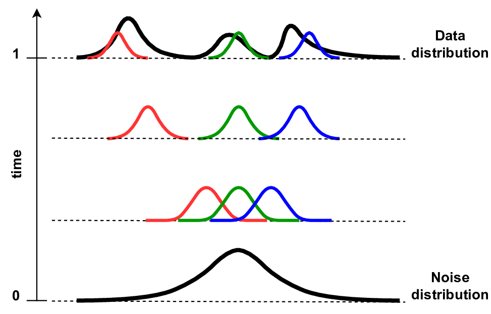
A
B
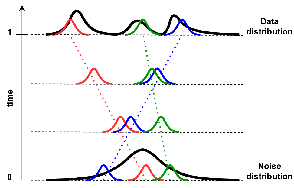
The differences between Lipman et al. CFM and Tong et al. iCFM are rather subtle. However, these subtle differences lead to different behavior of probability paths. In Figure 2, examples of these two CFMs are presented. Lipman at al. CFM starts with the standard Gaussian that evolves over time to a small Gaussian (i.e., standard deviation decreases) in the data space (see Figure 2A). Tong et al. CFM, on the other hand, defines a small Gaussian that is "moved" over time to the data space (see Figure 2B).
Training algorithms. We have all components necessary to define training of vector field models. The general algorithm is defined as follows:
- Sample $t \sim \text{Uniform}(0, 1)$.
- Sample $\mathbf{z} \sim q(\mathbf{z})$.
- Calculate $\mu_{t}(\mathbf{z})$ and $\sigma_{t}(\mathbf{z})$.
- Sample $\mathbf{x}_t \sim \mathcal{N}\left(\mathbf{x} | \mu(\mathbf{z}, t), \sigma(\mathbf{z}, t) \right)$.
- Calculate the vector field $v(\mathbf{x}_{t}, t; \mathbf{z})$.
- Calculate loss $\ell_{CFM}(\theta) = \| v_{\theta}(\mathbf{x}_t, t) - v(\mathbf{x}_{t}, t; \mathbf{z})\|^2$.
- Update parameters: $\theta \leftarrow \text{Update}\left(\theta, \nabla_{\theta} \ell_{CFM}(\theta) \right)$.
Depending on the choice of the mean function and the standard deviation function, we get a specific form of the vector field. Eventually, we obtain particular formulas in steps 3 and 5, while all other steps remain the same.
Sampling. Let me remind you, my curious reader, that we learn a model of the vector field. Once we have it, sampling is straightforward, namely:
- Sample $\mathbf{x} \sim q_0(\mathbf{x})$.
- Run forward Euler method until $t=1$ and with a step size $\Delta$: $$ \mathbf{x}_{t+\Delta} = \mathbf{x}_{t} + v_{\theta}(\mathbf{x}_{t}, t)\ \Delta .$$
Please note that in the case of flow matching, unlike in score-based generative models, we assume that time flows from $t=0$ (i.e., noise), to $t=1$ (i.e., data). As a result, once the model of the vector field is trained, we run the forward Euler method, not the backward Euler method like in score-based generative models.
Calculating the log-likelihood function. In the discussion on CNFs we showed that calculating the (log-)likelihood function is possible. Since flow matching does not require the log-likelihood function during training, we did not care about it so far. However, especially for evaluation, but also in many practical applications, being able to calculate the value of the log-likelihood function is beneficial. The full derivation of the log-likelihood function for flow matching is presented in Appendix C of (Lipman et al., 2022). The main idea is similar to CNFs and to make calculations practical, we use Hutchinson's trace estimator, that yields:
\begin{equation}\label{eq:loglikeli}\tag{2} \ln p_{1}(\hat{\mathbf{x}}_1) \approx \ln p_{0}(\hat{\mathbf{x}}_0) - f_{0} , \end{equation}
where $\hat{\mathbf{x}}_1$ is a data point, $\hat{\mathbf{x}}_0$ is noise that corresponds to $\hat{\mathbf{x}}_1$, and $f_{0}$ is an approximation of the trace of the vector field Jacobian. Note that we have only $\hat{\mathbf{x}}_1$, but we can obtain $\hat{\mathbf{x}}_0$ and $f_{0}$ by running the following procedure (Lipman et al., 2022):
- For given data point $\hat{\mathbf{x}}_1$, set the initial conditions: $$ \begin{bmatrix} \phi_1 \\ f_1 \end{bmatrix} = \begin{bmatrix} \hat{\mathbf{x}}_1 \\ 0 \end{bmatrix} . $$
- Define the following ODE:
$$
\frac{\mathrm{d}}{\mathrm{d}s}\begin{bmatrix}
\phi_{1-s} \\
f_{1-s}
\end{bmatrix} =
\begin{bmatrix}
-v_{\theta}(\phi_{1-s}, 1-s) \\
\epsilon^{\top} \nabla_{\phi} v_{\theta}(\phi_{1-s}, 1-s) \epsilon
\end{bmatrix}
$$
where $\epsilon \sim \mathcal{N}(0, \mathbf{I})$.
NOTE: We calculate $\nabla_{\phi} v_{\theta}(\phi_{1-s}, 1-s)$ by using autograd.
- Solve the ODE in step 2 by running the backward Euler method.
NOTE: Here we need to go from $t=1$ to $t=0$, thus, the backward Euler.
- Output the result: $$ \begin{bmatrix} \phi_0 \\ f_0 \end{bmatrix} = \begin{bmatrix} \hat{\mathbf{x}}_0 \\ \hat{c} \end{bmatrix} . $$
The outputs of this procedure are then plugged in to the equation (\ref{eq:loglikeli}) that yields:
\begin{equation}\label{eq:loglikelifinal}
\ln p_{1}(\hat{\mathbf{x}}_1) \approx \ln p_{0}(\hat{\mathbf{x}}_0) - \hat{c} .
\end{equation}
Please remember, my curious reader, that this is an approximation due to the trace estimator. However, the estimator is unbiased, and the variance can be reduced by running this procedure $M$ times for a given data point, and then averaging.
Coding flow matching
We outlined how to implement training and sampling (generation) using flow matching. The code is pretty straightforward and is outlined in the following code snippet. We picked the standard Gaussian noise distribution in our implementation, but please be aware that any other distribution would work.
The full code (with auxiliary functions) that you can play with is available here: link.
class FlowMatching(nn.Module):
    def __init__(self, vnet, sigma, D, T, stochastic_euler=False, prob_path="icfm"):
        super(FlowMatching, self).__init__()

        print('Flow Matching by JT.')

        self.vnet = vnet

        self.time_embedding = nn.Sequential(nn.Linear(1, D), nn.Tanh())

        # other params
        self.D = D

        self.T = T

        self.sigma = sigma

        self.stochastic_euler = stochastic_euler

        assert prob_path in ["icfm", "fm"], f"Error: The probability path could be either Independent CFM (icfm) or Lipman's Flow Matching (fm) but {prob_path} was provided."
        self.prob_path = prob_path

        self.PI = torch.from_numpy(np.asarray(np.pi))

    def log_p_base(self, x, reduction='sum', dim=1):
        log_p = -0.5 * torch.log(2. * self.PI) - 0.5 * x**2.
        if reduction == 'mean':
            return torch.mean(log_p, dim)
        elif reduction == 'sum':
            return torch.sum(log_p, dim)
        else:
            return log_p

    def sample_base(self, x_1):
        # Gaussian base distribution
        if self.prob_path == "icfm":
            return torch.randn_like(x_1)
        elif self.prob_path == "fm":
            return torch.randn_like(x_1)
        else:
            return None

    def sample_p_t(self, x_0, x_1, t):
        if self.prob_path == "icfm":
            mu_t = (1. - t) * x_0 + t * x_1
            sigma_t = self.sigma
        elif self.prob_path == "fm":
            mu_t = t * x_1
            sigma_t = t * self.sigma - t + 1.

        x = mu_t + sigma_t * torch.randn_like(x_1)

        return x

    def conditional_vector_field(self, x, x_0, x_1, t):
        if self.prob_path == "icfm":
            u_t = x_1 - x_0
        elif self.prob_path == "fm":
            u_t = (x_1 - (1. - self.sigma) * x) / (1. - (1. - self.sigma) * t)

        return u_t

    def forward(self, x_1, reduction='mean'):
        # =====Flow Matching
        # =====
        # z ~ q(z), e.g., q(z) = q(x_0) q(x_1), q(x_0) = base, q(x_1) = empirical
        # t ~ Uniform(0, 1)
        x_0 = self.sample_base(x_1)  # sample from the base distribution (e.g., Normal(0,I))
        t = torch.rand(size=(x_1.shape[0], 1))

        # =====
        # sample from p(x|z)
        x = self.sample_p_t(x_0, x_1, t)  # sample independent rv

        # =====
        # invert interpolation, i.e., calculate vector field v(x,t)
        t_embd = self.time_embedding(t)
        v = self.vnet(x + t_embd)

        # =====
        # conditional vector field
        u_t = self.conditional_vector_field(x, x_0, x_1, t)

        # =====LOSS: Flow Matching
        FM_loss = torch.pow(v - u_t, 2).mean(-1)

        # Final LOSS
        if reduction == 'sum':
            loss = FM_loss.sum()
        else:
            loss = FM_loss.mean()

        return loss

    def sample(self,  batch_size=64):
        # Euler method
        # sample x_0 first
        x_t = self.sample_base(torch.empty(batch_size, self.D))

        # then go step-by-step to x_1 (data)
        ts = torch.linspace(0., 1., self.T)
        delta_t = ts[1] - ts[0]

        for t in ts[1:]:
            t_embedding = self.time_embedding(torch.Tensor([t]))
            x_t = x_t + self.vnet(x_t + t_embedding) * delta_t
            # Stochastic Euler method
            if self.stochastic_euler:
                x_t = x_t + torch.randn_like(x_t) * delta_t

        x_final = torch.tanh(x_t)
        return x_final

    def log_prob(self, x_1, reduction='mean'):
        # backward Euler (see Appendix C in Lipman's paper)
        ts = torch.linspace(1., 0., self.T)
        delta_t = ts[1] - ts[0]

        for t in ts:
            if t == 1.:
                x_t = x_1 * 1.
                f_t = 0.
            else:
                # Calculate phi_t
                t_embedding = self.time_embedding(torch.Tensor([t]))
                x_t =x_t - self.vnet(x_t + t_embedding) * delta_t

                # Calculate f_t
                # approximate the divergence using the Hutchinson trace estimator and the autograd
                self.vnet.eval()  # set the vector field net to evaluation

                x = torch.FloatTensor(x_t.data)  # copy the original data (it doesn't require grads!)
                x.requires_grad = True

                e = torch.randn_like(x)  # epsilon ~ Normal(0, I)

                e_grad = torch.autograd.grad(self.vnet(x).sum(), x, create_graph=True)[0]
                e_grad_e = e_grad * e
                f_t = e_grad_e.view(x.shape[0], -1).sum(dim=1)

                self.vnet.eval()  # set the vector field net to train again

        log_p_1 = self.log_p_base(x_t, reduction='sum') - f_t

        if reduction == "mean":
            return log_p_1.mean()
        elif reduction == "sum":
            return log_p_1.sum()
Before we present results of generated images, let us see how flow matching behaves on the two moon dataset in Figure 3. We start with data generated according to the standard Gaussian, and then the vector field model (blue arrows) pushes the points towards two orange half-moons.
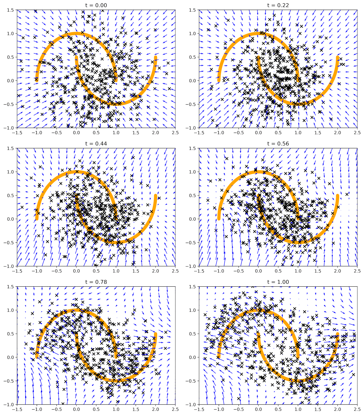
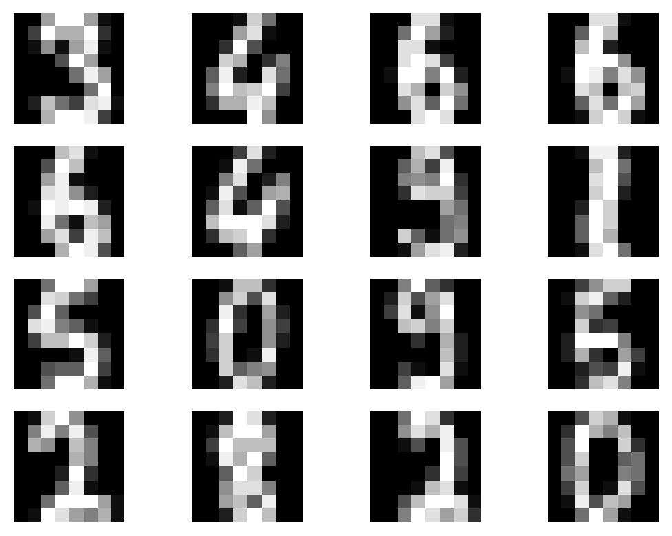
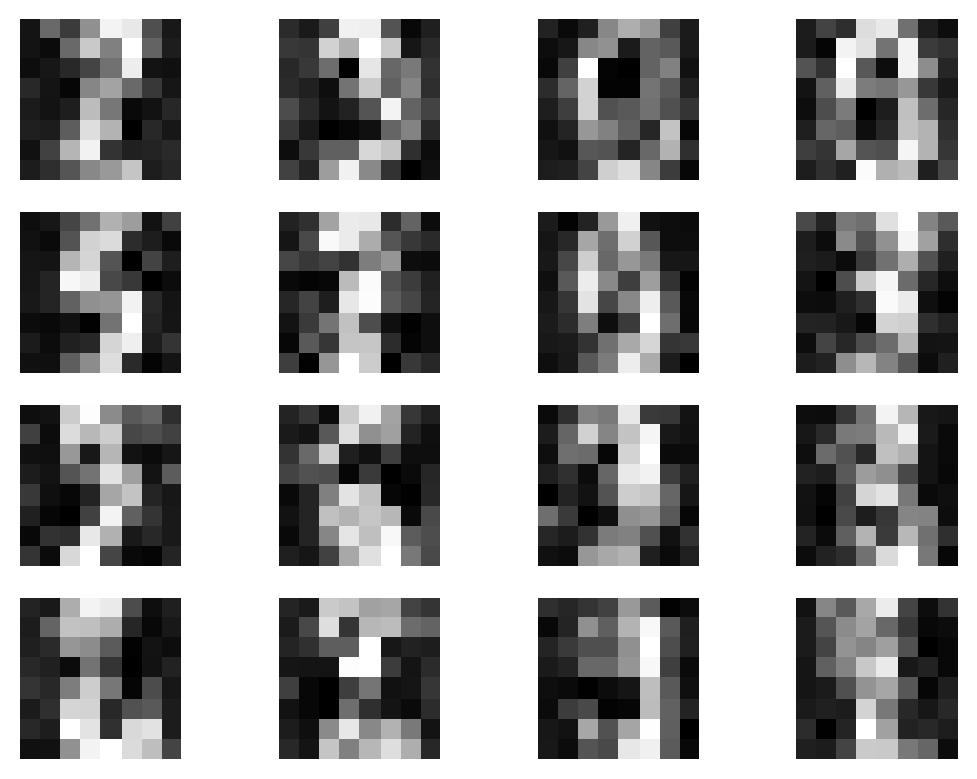
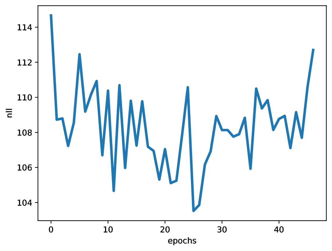
After running the code with an MLP-based vector field model, and the following values of the hyperparameters: $\sigma_{const} = 0.1$ and $T=100$, we can expect results like in Figure 4. Note that we report the negative log-likelihood estimated according to the procedure presented before.
A
B
C
What is the future of flow matching?
Flow matching is a framework first outlined in (Lipman et al., 2022), published in the fall of 2022. Since then, there are multiple extensions proposed. Here, I will point out a few but I highly recommend to search for new development, my curious reader, because I find this framework especially interesting!
Alright, let me attract your attention to the following papers:
- Similalry to Latent Diffusion, in (Dao et al., 2023) flow matching is used as a "prior" in an auto-encoder setting. First, the auto-encoder is trained, and then the vector field model is trained in the latent space. Afterwards, a sample from the FM model is decoded back to the data space.
- The idea of interpolations in CFM was further extented to stochastic interpolants proposed by (Albergo et al., 2023a; Albergo et al., 2023b). I highly recommend to look these papers up since they provide many interesting extensions, both theoretical and practical.
- As I mentioned earlier, one can propose a better distribution $q(\mathbf{z})$ by using Optimal Transport (OT). This results in OT-CFM (Tong et al., 2023) and Schrodinger Bridge CFM (De Bortoli et al., 2021; Vargas et al., 2021).
- Action matching, a closely related approach to CFM, proposed by (Neklyudov et al., 2023), allows learning an underlying mechanism of moving points in time without modeling the distributions at each step.
- Here, we considered interpolations in Euclidean spaces. (Chen & Lipman, 2023) proposed and extension of CFMs to general Riemannian manifolds.
- To take advantage of symmetries in data, (Klein et al., 2023) modified the cost function in OT-CFM to account for those. Additionally, they used equivariant graph neural networks to formulate equivariant flow matching.
- Here, we discussed the case of continuous random variables. However, in practice, we often deal with discrete data, e.g., molecules, proteins, pixel values. (Campbell et al., 2024) proposed Discrete Flow Models that could be seen as a version of CFM for handling discrete data.
- CFM was also proposed as an method for simulation-based inference (Wildberger et al., 2023), i.e., a problem in which one has an access to a simulator but the likelihood function is unknown or intractable.
- There are very close connections between score-based generative models and flow matching. I highly recommend looking into (Tong et al., 2023) and (Kingma & Gao, 2023) (the appendix therein is simply marvelous!) for further details.
There are multiple amazing papers that I missed, but I did not do that on purpose. It is simply very difficult to follow all of them. This statement is also a testament that flow matching is becoming the mainstream research direction in Generative AI. In my opinion, it is a fascinating framework that could bring multiple breakthroughs!
References
(Albergo et al., 2023a) Albergo, M. S., Boffi, N. M., & Vanden-Eijnden, E. (2023). Stochastic interpolants: A unifying framework for flows and diffusions. arXiv preprint arXiv:2303.08797.
(Albergo et al., 2023b) Albergo, M. S., Goldstein, M., Boffi, N. M., Ranganath, R., & Vanden-Eijnden, E. (2023). Stochastic interpolants with data-dependent couplings. arXiv preprint arXiv:2310.03725.
(Ben-Hamu et al., 2022) Ben-Hamu, H., Cohen, S., Bose, J., Amos, B., Grover, A., Nickel, M., Chen, R.T. and Lipman, Y., 2022. Matching normalizing flows and probability paths on manifolds. arXiv preprint arXiv:2207.04711.
(Campbell et al., 2024) Campbell, A., Yim, J., Barzilay, R., Rainforth, T., & Jaakkola, T. (2024). Generative Flows on Discrete State-Spaces: Enabling Multimodal Flows with Applications to Protein Co-Design. arXiv preprint arXiv:2402.04997.
(Chen et al., 2018) Chen, R.T., Rubanova, Y., Bettencourt, J. and Duvenaud, D.K., 2018. Neural ordinary differential equations. Advances in neural information processing systems, 31.
(Chen & Lipman, 2023) Chen, R. T., & Lipman, Y. (2023). Riemannian flow matching on general geometries. arXiv preprint arXiv:2302.03660.
(Dao et al., 2023) Dao, Q., Phung, H., Nguyen, B., & Tran, A. (2023). Flow matching in latent space. arXiv preprint arXiv:2307.08698.
(De Bortoli et al., 2021) De Bortoli, V., Thornton, J., Heng, J., & Doucet, A. (2021). Diffusion Schrödinger bridge with applications to score-based generative modeling. Advances in Neural Information Processing Systems, 34, 17695-17709.
(Grathwohl et al., 2018) Grathwohl, W., Chen, R.T., Bettencourt, J., Sutskever, I. and Duvenaud, D., 2018, September. FFJORD: Free-Form Continuous Dynamics for Scalable Reversible Generative Models. In International Conference on Learning Representations.
(Kingma & Gao, 2023) Kingma, D.P. and Gao, R., 2023, November. Understanding diffusion objectives as the ELBO with simple data augmentation. In Thirty-seventh Conference on Neural Information Processing Systems.
(Klein et al., 2023) Klein, L., Krämer, A., & Noé, F. (2023). Equivariant flow matching. Advances in Neural Information Processing Systems, 36.
(Lipman et al., 2022) Lipman, Y., Chen, R. T., Ben-Hamu, H., Nickel, M., & Le, M. (2022). Flow matching for generative modeling. arXiv preprint arXiv:2210.02747.
(Neklyudov et al., 2023) Neklyudov, K., Severo, D., & Makhzani, A. (2023). Action matching: A variational method for learning stochastic dynamics from samples. ICML 2023.
(Tong et al., 2023) Tong, A., Malkin, N., Huguet, G., Zhang, Y., Rector-Brooks, J., Fatras, K., ... & Bengio, Y. (2023). Improving and generalizing flow-based generative models with minibatch optimal transport. arXiv preprint arXiv:2302.00482.
(Vargas et al., 2021) Vargas, F., Thodoroff, P., Lamacraft, A., & Lawrence, N. (2021). Solving schrödinger bridges via maximum likelihood. Entropy, 23(9), 1134.
(Wildberger et al., 2023) Wildberger, J., Dax, M., Buchholz, S., Green, S., Macke, J. H., & Schölkopf, B. (2023). Flow Matching for Scalable Simulation-Based Inference. Advances in Neural Information Processing Systems, 36.