A Crash Course in Diffusion-based Models

An introduction to diffusion-based models

by Jakub Tomczak

Agenda

1. A quick recap on probabilistic theory and probabilistic modeling
2. Why (deep) generative modeling
3. Theory and code behind diffusion-based models

A recap on probabilistic theory

We will talk about random variables that we will denote by $\mathbf{x}$, $\mathbf{y}$, $\mathbf{z}$ and so on. We will define believes about states of random variables through probability distributions: (i) for discrete random variables, we will use probability mass functions, and (ii) for continuous random variables, we will use probability density functions. Either way, we will denote them as $p(\mathbf{x})$.

What we need to remember is that any joint distribution over random variables can be factorized in one of the two ways (product rule): \begin{align} p(\mathbf{x}, \mathbf{y}) &= p(\mathbf{x} | \mathbf{y})\ p(\mathbf{y}) \\ &= p(\mathbf{y} | \mathbf{x})\ p(\mathbf{x}) \end{align} and the marginal distribution can be calculated by marginalizing/summing out (sum rule): $$ p(\mathbf{x}) = \sum_{\mathbf{y}} p(\mathbf{x}, \mathbf{y}) $$

Funnily enough, these two rules are crucial for probabilistic modeling! Why? Think of Bayes rule: \begin{align} pp(\mathbf{y} | \mathbf{x})\ p(\mathbf{x}) &= \frac{p(\mathbf{x} | \mathbf{y})\ p(\mathbf{y})}{p(\mathbf{x})} \\ &= \frac{p(\mathbf{x} | \mathbf{y})\ p(\mathbf{y})}{\sum_{\mathbf{y}} p(\mathbf{x}, \mathbf{y})} \\ &= \frac{p(\mathbf{x} | \mathbf{y})\ p(\mathbf{y})}{\sum_{\mathbf{y}} p(\mathbf{x} | \mathbf{y})\ p(\mathbf{y})} \end{align}

A recap on probabilistic modeling

We assume some model, i.e., a probability distribution with some parameters $\theta$, $p(\mathbf{x}; \theta)$. For instance, for $x \in \{0, 1\}$ we pick a Bernoulli distribution: $$ p(x; \theta) = \theta^{x}\ (1 - \theta)^{1-x} ,$$ while for a continuous random variable ($x \in \mathbb{R}$), we can use a Normal (Gaussian) distribution with a mean/location $\mu$ and a standard deviation/scale $\sigma>0$): $$ p(x ; \theta = \{\mu, \sigma\}) = \frac{1}{\sqrt{2\pi \sigma^2}} \exp\left( -\frac{\left(x - \mu\right)^2}{2\sigma^2} \right) .$$

NOTE For the binary classification problem and the regression problem we DO use these two distributions! How? By modeling the conditional distribution $p(y|\mathbf{x})$ using, e.g., a neural network that outputs the parameters $\theta(\mathbf{x}) = \mathrm{NN}(x)$. If we take the logarithm of these two functions (and assume $\sigma=1$), we get the following: $$ \ln p(y; \theta(\mathbf{x})) = y \ln \theta(\mathbf{x}) + (1-y) \ln (1 - \theta(\mathbf{x})) $$ and $$\ln p(y; \theta(\mathbf{x})) = -\frac{1}{2}\left(y - \mu(\mathbf{x})\right)^2 + const .$$

Do these two quantities remind you of something? Let's rewrite them: $$ \ln p(y; \theta(\mathbf{x})) = \mathrm{BCE}\left(y, \theta(\mathbf{x})\right) , $$ and $$\ln p(y; \theta(\mathbf{x})) = -\frac{1}{2}\mathrm{MSE}\left(y, \mu(\mathbf{x})\right) + const .$$

The take-away is this: The log-probability of at least some distributions are equivalent to well-known loss functions in deep learning. And, consequently, we can think in terms of probability distributions to learn neural networks!

For given iid (identically, i.e., from the same distribution, and indepedently, i.e., all objects are observed independently, distributed) data $\mathcal{D} = \{\mathbf{x}_{n}\}_{n=1}^{N}$, we can calculate the likelihood function that assess what is the likelihood of observing data for given values of parameters $\theta$, namely: $$ p(\mathcal{D} | \theta) \stackrel{iid}{=} \prod_{n=1}^{N} p_{\theta}(\mathbf{x}_{n}) .$$

Equivalently, we can consider the logarithm of the likelihood function (the log-likelihood function): $$ \ln p(\mathcal{D} | \theta) = \sum_{n=1}^{N} \ln p_{\theta}(\mathbf{x}_{n}) ,$$ since the logarithm does not change the optimum.

Finding the best parameters of the model corresponds to maximizing the log-likelihood function or, equivalently, to minimizing the negative log-likelihood function: $$ \theta^{*} = \arg \min_{\theta} -\sum_{n=1}^{N} \ln p_{\theta}(\mathbf{x}_{n}) . $$

NOTE Interestingly, this optimization problem is equivalent to minimizing the Kullback-Leibler divergence between the data (empirical) distribution $p_{data}(\mathbf{x}) = \frac{1}{N} \sum_{n=1}^{N} \delta(\mathbf{x}_n)$ and the model distribution $p_{\theta}(\mathbf{x})$, namely: \begin{align} \mathrm{KL}\left[ p_{data}(\mathbf{x}) || p_{\theta}(\mathbf{x})\right] &= \int p_{data}(\mathbf{x}) \left[ \ln p_{data}(\mathbf{x}) - \ln p_{\theta}(\mathbf{x}) \right] \mathrm{d} \mathbf{x} \\ &= \underbrace{\int p_{data}(\mathbf{x}) \ln p_{data}(\mathbf{x}) \mathrm{d} \mathbf{x}}_{const} - \int p_{data}(\mathbf{x}) \ln p_{\theta}(\mathbf{x}) \mathrm{d} \mathbf{x} \\ &= const - \int p_{data}(\mathbf{x}) \ln p_{\theta}(\mathbf{x}) \mathrm{d} \mathbf{x} \\ &= const - \frac{1}{N} \sum_{n=1}^{N} \ln p_{\theta}(\mathbf{x}_{n}) . \end{align}

As you can see, minimizing the negative log-likelihood and minimizing the KL divergence between $p_{data}(\mathbf{x}) = \frac{1}{N} \sum_{n=1}^{N} \delta(\mathbf{x}_n)$ and $p_{\theta}(\mathbf{x})$ is the same!

How to build diffusion models

The ''Why'' behind (deep) generative modeling

There is a beautiful quote from the abstract of (Song et al., 2020):

"Creating noise from data is easy; creating data from noise is generative modeling."

This could be schematically presented in the following figure.

In other words, we can build the following probabilistic model:

1. Assume a distribution over noise, i.e., a distribution we can easily sample noise from, $p(noise)$.
2. Formulate a model that turns this noise into data, $p_{\theta}(\mathbf{x} | noise)$.

But remember, we think in a probabilistic manner, therefore, we should get rid of (a.k.a. marginalize out) the noise! In other words: $$ p(\mathbf{x}) = \int p(\mathbf{x} | noise)\ p(noise)\ \mathrm{d}\ noise .$$

We need to figure out how to take care of three aspects:

1. How to model noise!
2. How to model data given noise!
3. How to take care of the integral (sum)!

Modeling noise

Let us introduce latent variables $\mathbf{z}_{t}$, $t=1, 2, \ldots, T$ in a very specific manner. The last latent variable, $\mathbf{z}_{T}$, is sampled from the standard Gaussian distribution, $\mathbf{z}_{T} \sim \mathcal{N}(0, \mathbf{I})$. All other latent variables are generated through the following process: $$ p_{\theta}(\mathbf{z}_{1}, \ldots, \mathbf{z}_{T}) = \left( \prod_{t=1}^{T-1} p_{\theta}(\mathbf{z}_{t} | \mathbf{z}_{t+1}) \right)\ p(\mathbf{z}_{T}) . $$

We parameterize each distribution using a shared neural network that takes $\mathbf{z}_{t+1}$ and $t$ as inputs. It might sound weird put it will become more obvious (hopefully!) later on.

We don't impose any interpretation on the latent variables $\mathbf{z}_{1}, \ldots, \mathbf{z}_{T-1}$ for now, but intuitively we can say they represent some intermediatery steps between data and noise. Again, hopefully, this will become clear in a second!

Modeling data

Further, once we sampled all latents, we can generate data using the conditional distribution $p_{\psi}(\mathbf{x} | \mathbf{z}_1)$. If our data live in $\mathbb{R}^{D}$, then we can pick another Gaussian: $p_{\psi}(\mathbf{x} | \mathbf{z}_1) = \mathcal{N} \left( \mathbf{x} | \{\mu, \sigma\} = \mathrm{NN}_{\psi}(\mathbf{z}_{1}) \right)$. For other distributions, we can use a similar trick (but for some cases, we need to fulfill additional requirements).

Dealing with the integral: Variational inference

Variational Inference (VI) is an approximate inference method that defines a (parametric) family of variational distributions approximating exact posteriors. In our case, this would correspond to $q_{\phi}(noise | \mathbf{x})$. Then, we can re-formulate the integral as follows: \begin{align} p(\mathbf{x}) &= \int p(\mathbf{x} | noise)\ p(noise)\ \mathrm{d}\ noise \\ &= \int \frac{q_{\phi}(noise | \mathbf{x})}{q_{\phi}(noise | \mathbf{x})} p(\mathbf{x} | noise)\ p(noise)\ \mathrm{d}\ noise \\ &\geq \int q_{\phi}(noise | \mathbf{x}) \frac{ p(\mathbf{x} | noise)\ p(noise)}{q_{\phi}(noise | \mathbf{x})}\ \mathrm{d}\ noise \\ &= \mathbb{E}_{noise \sim q_{\phi}(noise | \mathbf{x})}\left[ \frac{ p(\mathbf{x} | noise)\ p(noise)}{q_{\phi}(noise | \mathbf{x})} \right] \end{align} The resulting lower bound is called the Evidence Lower Bound (ELBO).

Now, taking the logarithm and then applying Jensen's inequality yields: \begin{align} \ln p(\mathbf{x}) &\geq \ln \mathbb{E}_{noise \sim q_{\phi}(noise | \mathbf{x})}\left[ \frac{ p(\mathbf{x} | noise)\ p(noise)}{q_{\phi}(noise | \mathbf{x})} \right] \\ &= \mathbb{E}_{noise \sim q_{\phi}(noise | \mathbf{x})}\left[ \ln p(\mathbf{x} | noise) + \ln p(noise) - \ln q_{\phi}(noise | \mathbf{x}) \right] \end{align}

We haven't done much, we still have the integral there, and, additionally, we have a lower bound, but at least we can approximate this integral by sampling from $q_{\phi}(noise | \mathbf{x})$. If we can sample efficiently (and, ideally, with a low variance), then we can use Monte Carlo methods to approximate the integral efficiently. Moreover, take a look that we can calculate the log-likelihood function here! This is what we want to optimize after all!

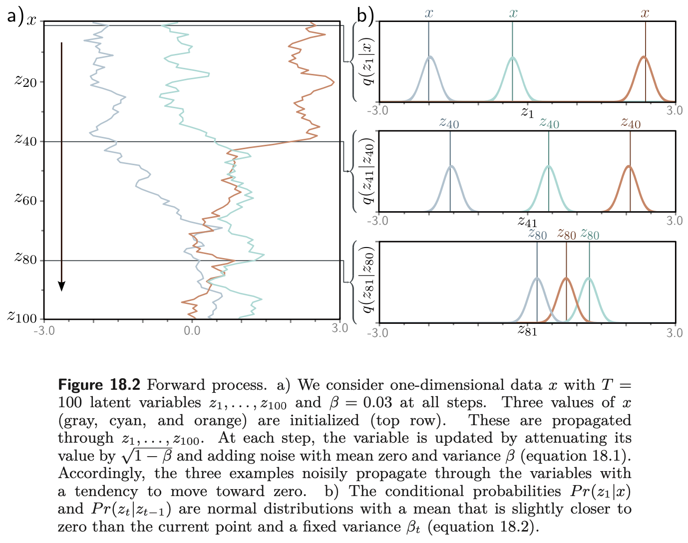
Now, coming back to our approach. We want to define multiple levels of noise. In other words, we can pick a specific family of variational distributions that turn data into Gaussian noise in the following recursive manner: $$ \mathbf{z}_t = \sqrt{1 - \beta_t} \mathbf{z}_{t-1} + \sqrt{\beta_t} \epsilon_t , $$ where $\beta_t < 1$ is the variance, and $\epsilon_t \sim \mathcal{N}(0, \mathbf{I})$. If you are familiar with the reparameterization trick, this corresponds to the following vartiational posterior: $$ q(\mathbf{z}_{t} | \mathbf{z}_{t-1}) = \mathcal{N}(\mathbf{z}_{t} | \sqrt{1 - \beta_t} \mathbf{z}_{t-1}, \beta_t \mathbf{I}). $$

Since this is the linear Gaussian model, it is also possible to calculate the following distribution (if you don't believe me, check it out yourself!): $$ q(\mathbf{z}_{t} | \mathbf{x}) = \mathcal{N}(\mathbf{z}_{t} | \sqrt{\alpha_t} \mathbf{x}, (1 - \alpha_t) \mathbf{I}) ,$$ where $\alpha_t = \prod_{s = 1}^{t} (1 - \beta_{s})$.

Having this distribution is AMAZING because we can sample any level of noisy data in a SINGLE STEP!

Interestingly, we can also calculate the following variational distribution exactly (following the linear Gaussian model again): $$ q(\mathbf{z}_{t} | \mathbf{z}_{t+1}, \mathbf{x}) = \mathcal{N}(\mathbf{z}_{t} | \mu_{t}(\mathbf{x}, \mathbf{z}_{t+1}), \sigma_{t}^{2} \mathbf{I}) ,$$ where: \begin{align} \mu_{t}(\mathbf{x}, \mathbf{z}_{t+1}) &= \frac{1}{1 - \alpha_{t+1}} \left( (1 - \alpha_t) \sqrt{1 - \beta_{t+1}} \mathbf{z}_{t+1} + \sqrt{\alpha_t} \beta_{t+1} \mathbf{x} \right) \\ \\ \sigma_{t}^{2} &= \frac{\beta_{t+1}(1 - \alpha_t)}{1 - \alpha_{t+1}} \end{align}

We can plug this in to the ELBO and after a few modifications, we get the following lower bound: \begin{align} &\geq \mathbb{E}_{\mathbf{z}_{1:T} \sim q(\mathbf{z}_{1:T} | \mathbf{x})}\left[ \ln p(\mathbf{x} | \mathbf{z}_{1}) + \sum_{t=1}^{T-1} \ln p(\mathbf{z}_{t} | \mathbf{z}_{t+1}) + \ln p(\mathbf{z}_{T}) + \right.\\ &\left. - \sum_{t=1}^{T-1} \ln q(\mathbf{z}_{t} | \mathbf{z}_{t+1}, \mathbf{x}) - \ln q(\mathbf{z}_{T} | \mathbf{x}) \right] \\ &= \mathbb{E}_{\mathbf{z}_{1:T} \sim q(\mathbf{z}_{1:T} | \mathbf{x})}\left[ \underbrace{\ln p(\mathbf{x} | \mathbf{z}_{1})}_{L_0} + \sum_{t=1}^{T-1} \underbrace{\left\{ \ln p(\mathbf{z}_{t} | \mathbf{z}_{t+1}) - \ln q(\mathbf{z}_{t} | \mathbf{z}_{t+1}, \mathbf{x})\right\}}_{L_t} + \right.\\ &\left. \underbrace{\ln p(\mathbf{z}_{T}) - \ln q(\mathbf{z}_{T} | \mathbf{x})}_{L_T} \right] \end{align}

Nice! However, can we really train a model like that? Especially if we take $T$ equal, say, 1000? Not really... But we can be smart about it!

Putting it all together: Diffusion-based models

Before we do smart things, let us recap the whole approach:

• We have latent variables that go from pure noise, $\mathbf{z}_T$, to data, $\mathbf{x}$.
• Each latent variable is defined as an interpolation between data and noise, $\epsilon_t \sim \mathcal{N}(0, \mathbf{I})$, namely: $$ \mathbf{z}_{t} = \sqrt{\alpha_t} \mathbf{x} + \sqrt{1 - \alpha_t} \epsilon_t .$$
• We have a generative model parameterized by a shared neural network, namely, every $p(\mathbf{z}_{t} | \mathbf{z}_{t+1})$ is parameterized by the same neural network.
• For the chosen variational posteriors, i.e., linear Gaussian models, we can derive the ELBO.
• The resulting approach is a discrete-time diffusion model with Gaussian diffusion in the forward process (i.e., from data to noise), and a non-linear diffusion in the backward process (i.e., from noise to data).
• This model is basically a Variational Auto-Encoder: (i) it is a hierarchical model, (ii) $\forall_t\ \mathrm{dim}(\mathbf{z}_{t}) = \mathrm{dim}(\mathbf{x})$, (iii) the encoder is a linear Gaussian model, (iv) the decoder shares the same neural network across all stochastic levels.

So far, we prepared good foundations for formulating a scalable and efficient generative model. However, there are still a few points missing:

• The essential point is that to train this model, we don't need to optimize the full ELBO. Since we train using a stochastic gradient-based optimizer, it is fine to sample $t$ uniformly and update the model accordingly. This releases us from storing all $T$ latents and corresponding losses, and makes the updates much lighter! However, this is only possible if we share the same neural network across all layers. Now you see why we mentioned that before.
• If we assume all distributions in the backward process to be Gaussians, we can notice the following: \begin{align} L_{t}(\mathrm{NN}) &= \mathbb{E}_{\mathbf{z}_{1:T} \sim q(\mathbf{z}_{1:T} | \mathbf{x})}\left[ \ln p(\mathbf{z}_{t} | \mathbf{z}_{t+1}) - \ln q(\mathbf{z}_{t} | \mathbf{z}_{t+1}, \mathbf{x}) \right] \\ &= \frac{1}{2\beta_t} \| \mu_{t}(\mathbf{x}, \mathbf{z}_{t+1}) - \mathrm{NN}(\mathbf{z}_{t+1}, t) \|^{2} + const . \end{align}

Further, we can realize that we can change the role of the neural network from predicting the parameters of a distribution to predicting the noise added to latents $\mathbf{z}_{t}$. We can express a datapoint $\mathbf{x}$ using the latents and the noise as follows: $$ \mathbf{x} = \frac{1}{\sqrt{\alpha_t}} \mathbf{z}_{t} - \frac{\sqrt{1 - \alpha_t}}{\sqrt{\alpha_t}} \epsilon_t $$ and by plugging it to the mean function $\mu_{t}(\mathbf{x}, \mathbf{z}_{t+1})$, we can re-express $L_{t}$ as follows: \begin{align} L_{t}(\mathrm{NN}) &= \frac{\beta_t}{2(1-\alpha_t)(1-\beta_t)} \| \mathrm{NN}(\mathbf{z}_{t+1}, t) - \epsilon_t \|^{2} + const . \end{align}

Further, we can even skip the scaling and optimize the $\ell_2$-norm term alone, namely: \begin{align} L_{t, simple}(\mathrm{NN}) &= \| \mathrm{NN}(\mathbf{z}_{t+1}, t) - \epsilon_t \|^{2} . \end{align} In the literature, it is called the simple loss.

Training

Now we can finally pull off with a training step:

1. Sample a datapoint $\mathbf{x} \sim p_{data}$.
2. Sample a timestep, $t \sim \mathcal{U}[1, \ldots, T]$.
3. Sample a noise vector, $\epsilon_t \sim \mathcal{N}(0, \mathbf{I})$.
4. Sample a noisy image, $\mathbf{z}_{t} = \sqrt{\alpha_t} \mathbf{x} + \sqrt{1 - \alpha_t} \epsilon_t$.
5. Compute the simple loss term: $L_{t}(NN) = \| \mathrm{NN}(\mathbf{z}_{t}, t) - \epsilon_t \|^2$.
6. Apply the optimizer step for the loss in 5.

Some important remarks:

• First, the neural network is shared across all levels. Note that to make it aware of the point along the diffusion process, it take as input the timestep $t$ as well. We need to handle it properly.
• Second, we update the neural network for a single $L_t$, not the full ELBO. Since we use a stochastic graadient-based optimizer, it basically doesn't matter!
• Third, in practice, it turns out that the simple loss works just fine. One of the reasons is that if we use ADAM or other adaptive gradient-based methods, the scaling factor doesn't play any role since the optimzer is capable of scaling its gradients.

Sampling (generating)

Once we trained a model, we can apply the backward diffusion to sample new datapoints:

1. Sample the final latent (i.e., noise), $\mathbf{z}_{T} \sim \mathcal{N}(0, \mathbf{I})$.
2. Sample noise, $\epsilon_t \sim \mathcal{N}(0, \mathbf{I})$.
3. Calculate a noisy image: $$\mathbf{z}_{t-1} = \underbrace{\frac{1}{\sqrt{1 - \beta_t}} \left( \mathbf{z}_{t} - \frac{\beta_t}{\sqrt{1 - \alpha_t}} \mathrm{NN}(\mathbf{z}_{t}, t) \right)}_{\mu(\mathbf{z}_{t}, t)} + \sqrt{\beta_t} \epsilon_{t}$$
4. Go to 2 unless $t$ equals 1, then: $$\mathbf{x} = \frac{1}{\sqrt{1 - \beta_1}} \left( \mathbf{z}_{1} - \frac{\beta_1}{\sqrt{1 - \alpha_1}} \mathrm{NN}(\mathbf{z}_{1}, 1) \right)$$

A schematic representation of sampling from diffusion models (Prince, 2024):

An example

Let us consider a single neural network that is a ResNet.

At each layer, we embedd time (in the same way!) and add it to the input vector.

For images, a U-Net architecture is typically used. Recently, a ViT architecture is used within the U-Net.

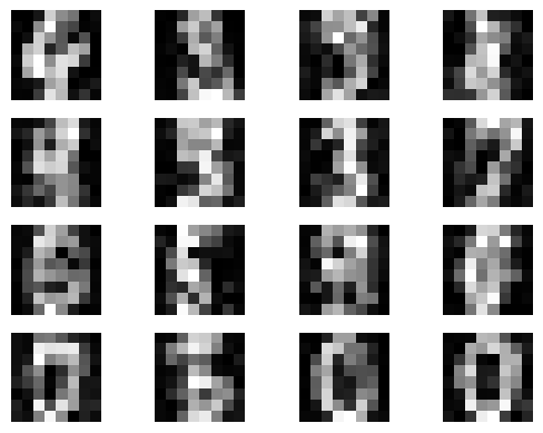
Let us take an extremely simple data: a sub-sampled (~2k images), and downscaled (8x8) MNIST. We transform them to be in $[-1, 1]$.

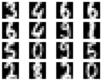
Training a diffusion-model with $T=10$, with a ResNet shared across all levels, can result in a model that generates the following images:

Thank you!