Agenda
- A reminder on diffusion models
- Stochastic/Ordinary Differential Equations as deep generative models
- PF-ODEs as score-based generative models
- An example: Variance Exploding PF-ODE
- Training and sampling
- An example
- Appendix
A reminder on diffusion-based models
We can think of a diffusion model as a dynamical system with discretized time.
Let $\mathbf{x}_0 \sim p_{0}(\mathbf{x}) \equiv p_{data}(\mathbf{x})$ denote noise, $\mathbf{x}_{1} \sim p_{1}(\mathbf{x}) \equiv \pi(\mathbf{x})$ is a sample from a known distribution, the "time" be denoted by $t \in [0, 1]$, and there are $T$ steps between $\mathbf{x}_{0}$ and $\mathbf{x}_{1}$, namely, a step size is $\Delta = \frac{1}{T}$. Then, we can represent the forward diffusion as follows:
\begin{equation} \mathbf{x}_{t+\Delta} = \sqrt{1 - \beta_t}\ \mathbf{x}_{t} + \sqrt{\beta_t}\ \epsilon_{t} , \end{equation}
where $\epsilon_{t} \sim \mathcal{N}(0, \mathbf{I})$.
We can learn a diffusion-based model by minimizing the KL-term or, even simpler, the MSE:
\begin{equation} \mathcal{L}_{t}(\theta) = \|\epsilon_{\theta}(\mathbf{x}_{t}, t) - \epsilon_{t}\|^{2}, \end{equation}
There exists the following correspondence between the score model and the noise model (for Gaussian denoising distribution with the standard deviation $\sigma$):
\begin{equation} s_{\theta}(\mathbf{x}, t) = -\frac{\epsilon_{\theta}(\mathbf{x}_{t}, t)}{\sigma} . \end{equation}
Let us sum these considerations up:
- The forward diffusion defines a discrete-time dynamical system.
- The loss function for diffusion-based models is (almost) identical to the score-matching loss.
- In fact, diffusion-based models correspond to score models.
- Diffusion-based models are very similar to score models trained with a schedule for $\sigma$ because both models are iterative and both models consider more noise at each step.
These similarities indicate that there may be an underlying framework that could generalize score models and diffusion-based models.
Stochastic/Ordinary Differential Equations as deep generative models
ODEs and numerical methods ODEs can be defined as follows:
\begin{equation} \frac{\mathrm{d} \mathbf{x}_t}{\mathrm{d} t} = f(\mathbf{x}_{t}, t) , \end{equation}
with some initial conditions $\mathbf{x}_{0}$. Sometimes, $f(\mathbf{x}_{t}, t)$ is referred to as a vector field.
We can solve this ODE by running one of the numerical methods that aims to discretize time in a specific way. For instance, Euler's method carries it out in the following way (starting from $t=0$ and proceeding to $t=1$ with a step $\Delta$):
\begin{align} \mathbf{x}_{t+\Delta} - \mathbf{x}_{t} &= f(\mathbf{x}_{t}, t) \cdot \Delta \\ \mathbf{x}_{t+\Delta} &= \mathbf{x}_{t} + f(\mathbf{x}_{t}, t) \cdot \Delta \end{align}
Sometimes, it is necessary to run from $t=1$ to $t=0$, then we can apply backward Euler's method:
\begin{equation} \mathbf{x}_{t} = \mathbf{x}_{t+\Delta} - f(\mathbf{x}_{t+\Delta}, t+\Delta) \cdot \Delta \end{equation}
If we take $\mathbf{x}_0$ to be our data, and $\mathbf{x}_{1}$ to be noise, then if we knew $f(\mathbf{x}_{t}, t)$, we could run backward Euler's method to get a generative model!
Please keep this thought in mind!
SDEs and Probability Flow ODEs In general, we can think of SDEs as ODEs whose trajectories are random and are distributed according to some probabilities at each $t$, $p_{t}(\mathbf{x})$. SDEs could be defined as follows:
\begin{equation} \mathrm{d} \mathbf{x}_{t} = f(\mathbf{x}_{t}, t) \mathrm{d} t + g(t) \mathrm{d} \mathbf{v}_{t} , \end{equation}
where $\mathbf{v}$ is a standard Wiener process, $f(\cdot, t)$ in this context is referred to as drift, and $g(\cdot)$ is a scalar function called diffusion.
The drift component is deterministic, but the diffusion element is stochastic due to the standard Wiener process (for more about Wiener processes, see (Särkkä & Solin, 2019); here, we do not need to know more than that they behave like Gaussians, e.g., the difference of its increments is normally distributed, $\mathbf{v}_{t+\Delta} - \mathbf{v}_{t} \sim \mathcal{N}(0,\Delta)$). A side note: The forms of drift and diffusion are assumed to be known.
An important property of this SDE is the existence of a corresponding ordinary differential equation whose solutions follow the same distribution! If we start with a datapoint $\mathbf{x}_0$, we can get noise $\mathbf{x}_1 \sim p_{1}(\mathbf{x})$ by solving the following Probability Flow (PF) ODE (Song et al., 2020):
\begin{equation} \frac{\mathrm{d} \mathbf{x}_{t}}{\mathrm{d} t} = \left( f(\mathbf{x}_{t}, t) - \frac{1}{2}g^{2}(t) \nabla_{\mathbf{x}_{t}} \ln p_{t}(\mathbf{x}_{t}) \right) . \end{equation}
Let us take another look at that and see what we got:
- First of all, we do not have the Wiener process anymore. As a result, we deal with an ODE instead of an SDE.
- Second, the drift component and the diffusion components are still here, but the diffusion is multiplied by $-\frac{1}{2}$ and squared.
- Third, there is the score function! If you want to see a derivation, please check (Song et al., 2020), here we take it for granted as true. However, it looks reasonable. SDEs have solutions that are distributed according to $p_{t}(\mathbf{x})$, hence, it is not surprising that the score function pops up here. After all, the score function indicates how a trajectory should look like according to $p_{t}(\mathbf{x})$.
PF-ODEs as score-based generative models
If we assume that the score function is known, we can use this PF-ODE as a generative model by applying backward Euler's method starting from $\mathbf{x}_{1} \sim \pi(\mathbf{x})$:
\begin{equation} \mathbf{x}_{t} = \mathbf{x}_{t+\Delta} - \left( f(\mathbf{x}_{t+\Delta}, t+\Delta) - \frac{1}{2}g^{2}(t+\Delta) \nabla_{\mathbf{x}_{t+\Delta}} \ln p_{t}(\mathbf{x}_{t+\Delta}) \right) \cdot \Delta . \end{equation}
We can learn using denoising score matching. The difference to denoising score matching is that we need to take time $t$ into account:
\begin{equation} \mathcal{L}(\theta) = \int_{0}^{1} \mathcal{L}_t(\theta) \mathrm{d} t . \end{equation}
The score matching method tells us that we should consider $\lambda_t \| s_{\theta}(\mathbf{x}_t, t) - \nabla_{\mathbf{x}_t} \ln p_{t}(\mathbf{x}_t) \|^2$, but since we cannot calculate $p_{t}(\mathbf{x}_t)$, we can define a distribution $p_{0t}(\mathbf{x}_t|\mathbf{x}_0)$ that allows sampling noisy versions of our original datapoints $\mathbf{x}_0$'s. Putting it all together yields:
\begin{equation} \mathcal{L}_t(\theta) = \frac{1}{2} \mathbb{E}_{\mathbf{x}_0 \sim p_{data}(\mathbf{x})} \mathbb{E}_{\mathbf{x}_t \sim p_{0t}(\mathbf{x}_t|\mathbf{x}_0)} \left[ \lambda_t \| s_{\theta}(\mathbf{x}_t, t) - \nabla_{\mathbf{x}_t} \ln p_{0t}(\mathbf{x}_t|\mathbf{x}_0) \|^2 \right] . \end{equation}
Importantly, if we take $p_{0t}(\mathbf{x}_t|\mathbf{x}_0)$ to be Gaussian, then we could calculate the score function analytically. Moreover, to calculate $\mathcal{L}_t(\theta)$, we can use a single sample (i.e., the Monte Carlo estimate).
After finding $s_{\theta}(\mathbf{x}_t, t)$, we can sample data by running backward Euler's method as follows:
\begin{equation} \mathbf{x}_{t} = \mathbf{x}_{t+\Delta} - \left( f(\mathbf{x}_{t+\Delta}, t+\Delta) - \frac{1}{2}g^{2}(t+\Delta) s_{\theta}(\mathbf{x}_{t+\Delta}, t + \Delta) \right) \cdot \Delta \end{equation}
Please keep in mind that drift and diffusion are assumed to be known. Additionally, we stick to (backward) Euler's method, but you can pick another ODE solver.
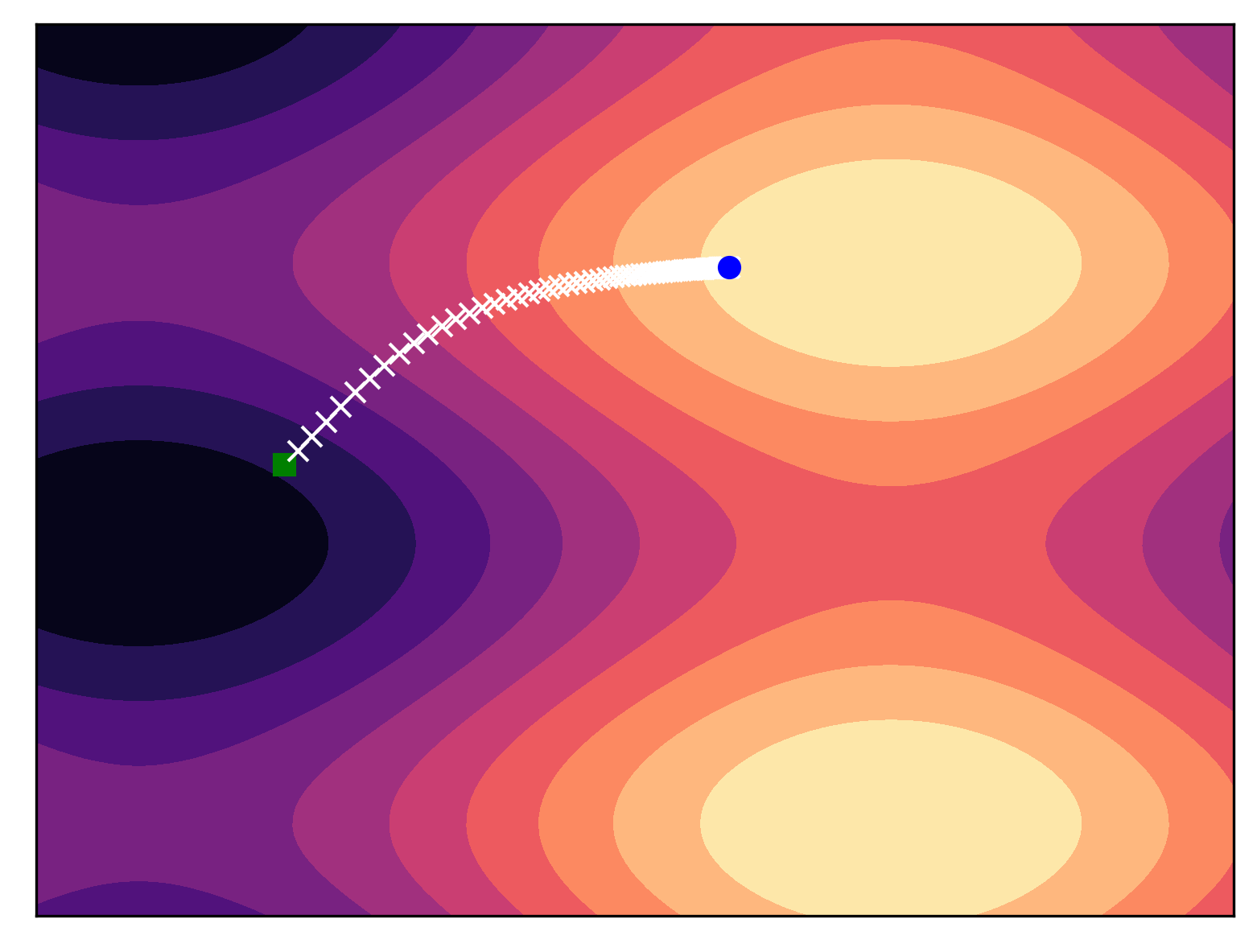
For some PF-ODE and a given score function, we can obtain samples from a multimodal distribution.T he ODE solver "goes" towards modes. In the following simple example, we can notice that defining PF-ODEs is a powerful generative tool! Once the score function is properly approximated, we can sample from the original distribution in a straightforward manner.
An example: Variance Exploding PF-ODE
To define our own score-based generative model (SBGM), we need the following elements:
- the drift $f(\mathbf{x}, t)$;
- the diffusion $g(t)$;
- and the form of $p_{0t}(\mathbf{x}_{t}|\mathbf{x}_0)$.
In (Song et al., 2020) and (Song et al., 2021), we can find three examples of SGBMs, namely, Variance Exploding (VE) SDE, Variance Preserving SDE, and sub-VP SDE. Here, we focus on the VE SDE.
In the VE SDE, we consider the following choices of the drift and the diffusion:
- $f(\mathbf{x}, t) = 0$,
- $g(t) = \sigma^{t}$, where $\sigma > 0$ is a hyperparameter; note that we take $\sigma$ to the power of time $t \in [0,1]$.
Then, according to our discussion above, plugin our choices for $f(\mathbf{x}, t)$ and $g(t)$ in the general form of the PF-ODE yields:
\begin{equation} \frac{\mathrm{d} \mathbf{x}_{t}}{\mathrm{d} t} = - \frac{1}{2} \sigma^{2t} \nabla_{\mathbf{x}_t} \ln p_{t}(\mathbf{x}_{t}) . \end{equation}
Now, to learn the score model, we need to define the conditional distribution for obtaining a noisy version of $\mathbf{x}_0$.
The theory of SDEs (e.g., see Chapter 5 of (Särkkä & Solin, 2019)) tells us how to calculate $p_{0t}(\mathbf{x}_{t}|\mathbf{x}_0)$. Specific formulas are presented in the Appendix of (Song et al., 2020). Here we provide the final solution:
\begin{equation} p_{0t}(\mathbf{x}_{t}|\mathbf{x}_0) = \mathcal{N}\left(\mathbf{x}_t | \mathbf{x}_0, \frac{1}{2 \ln \sigma}(\sigma^{2t} - 1) \mathbf{I}\right) , \end{equation}
thus, the variance function over time is the following:
\begin{equation} \sigma_t^2 = \frac{1}{2 \ln \sigma}(\sigma^{2t} - 1). \end{equation}
Eventually, the final distribution, $p_{01}(\mathbf{x})$ gets approximately close to the following Gaussian (for sufficiently large $\sigma$):
\begin{align} p_{01}(\mathbf{x}) &= \int p_{0}(\mathbf{x}_0) * \mathcal{N} \left( \mathbf{x} | \mathbf{x}_{0}, \frac{1}{2 \ln \sigma}(\sigma^{2} - 1)\mathbf{I} \right) \\ &\approx \mathcal{N}\left( \mathbf{x} | 0, \frac{1}{2 \ln \sigma}(\sigma^{2} - 1)\mathbf{I} \right) . \end{align}
We will use $p_{01}(\mathbf{x})$ to sample noise $\mathbf{x}_1$ and then for reverting it to data $\mathbf{x}_0$.
Training of SBDMs
Traning consists of the following steps:
- Pick a datapoint $\mathbf{x}_0$.
- Sample $\mathbf{x}_1 \sim \pi(\mathbf{x}) = \mathcal{N}\left( \mathbf{x} | 0, \mathbf{I} \right)$.
- Sample $t \sim \mathrm{Uniform}(0,1)$.
- Calculate $\mathbf{x}_t = \mathbf{x}_0 + \sqrt{\frac{1}{2 \ln \sigma}(\sigma^{2t} - 1)} \cdot \mathbf{x}_{1}$. This is a sample from $p_{0t}(\mathbf{x}_{t}|\mathbf{x}_{0})$.
- Evaluate the score model at $\mathbf{x}_t$ and $t$, $s_{\theta}(\mathbf{x}_t, t)$.
- Calulate the score matching loss for a single sample, $\mathcal{L}_{t}(\theta) = \sigma_{t}^2 \| \mathbf{x}_1 - \sigma_t s_{\theta}(\mathbf{x}_t, t) \|^2$.
- Update $\theta$ using a gradient-based method with $\nabla_{\theta} \mathcal{L}_{t}(\theta)$.
We repeat these 7 steps for available training data until some stop criterion is met. Obviously, in practice, we use mini-batches instead of single datapoints.
In this training procedure we use $-\sigma_t s_{\theta}(\mathbf{x}_t, t)$ on purpose because $-\sigma_t s_{\theta}(\mathbf{x}_t, t) = \epsilon_{\theta}(\mathbf{x}_t, t)$ and then the criterion $\sigma_{t}^2 \| \mathbf{x}_1 - \epsilon_{\theta}(\mathbf{x}_t, t) \|^2$ corresponds to diffusion-based models (Kingma et al., 2021; Kingma & Gao, 2023).
Sampling
After training the score model, we can generate by running backward Euler's method (or other ODE solvers that takes the following form for the VE PF-ODE:
\begin{align} \mathbf{x}_{t} &= \mathbf{x}_{t+\Delta} + \left( \frac{1}{2}\sigma^{2(t+\Delta)} \left\{ - \frac{1}{\sigma^{t+\Delta}} s_{\theta}(\mathbf{x}_{t+\Delta}, t + \Delta) \right\} \right) \cdot \Delta \\ &= \mathbf{x}_{t+\Delta} - \left( \frac{1}{2}\sigma^{t+\Delta} s_{\theta}(\mathbf{x}_{t+\Delta}, t + \Delta) \right) \cdot \Delta \end{align}
starting from $\mathbf{x}_1 \sim p_{01}(\mathbf{x}) = \mathcal{N}\left( \mathbf{x} | 0, \frac{1}{2 \ln \sigma}(\sigma^{2} - 1)\mathbf{I} \right)$.
Note that in the first line, we have the plus sign because the diffusion for the VE PF-ODE is $-\frac{1}{2} \sigma^{2t}$; therefore, the minus sign in backward Euler's method turns to plus.
An example
After running the code with an MLP-based scoring model and the following values of the hyperparameters $\sigma = 1.01$ and $T=20$, we can expect results like in the figure below:

Appendix
Other SBGMs There are other classes of SBGMs besides Variance Exploding, namely (Song et al., 2020):
- Variance Preserving (VP): the drift is $f(\mathbf{x}, t) = - \frac{1}{2} \beta_t \mathbf{x}$, the diffusion is $g(t) = \sqrt{\beta_t}$, and the loss weighting is $\lambda_t = 1 - \exp\{- \int_{0}^{t} \beta_s \mathrm{d}s\}$, where $\beta_t$ is some function of time $t$.
- sub-VP: the drift is $f(\mathbf{x}, t) = - \frac{1}{2} \beta_t \mathbf{x}$, the diffusion is $g(t) = \sqrt{\beta_t \left( 1 - \exp\{- 2\int_{0}^{t} \beta_s \mathrm{d}s\} \right)}$, and the loss weighting is $\lambda_t = \left( 1 - \exp\{- \int_{0}^{t} \beta_s \mathrm{d}s\} \right)^2$, where $\beta_t$ is some function of time $t$.
There exist various versions of these models, especially there are different ways of defining $\lambda_t$ and other functions dependent on $t$ like $\sigma_t$ in VE and $\beta_t$ in VP. See (Kingma & Gao, 2023) for an overview.
Better solvers One drawback of SBGMs is the large number of steps during sampling. (Lu et al., 2022) presented specialized ODE solvers that could achieve great performance within $T=10$, which was further improved to $T=5$ (Zhou et al., 2023)! A better-suited solver could be used to obtain better results, e.g., by using Heun's method (Karras et al., 2022).
Other improvements There are many ideas within the domain of score-based models! Here, I will name only a few:
- Using SBGMs in the latent space (Vahdat et al., 2021).
- In fact, it is possible to calculate the log-likelihood function for SBGMs in a similar manner to neural ODE (Chen et al., 2018). (Song et al., 2021) showed that the log-likehood function could be upper-bounded by some modification of the score matching loss.
- Using various tricks to improve the log-likelihood estimation like dequantization and importance-weighting (Zheng et al., 2023).
- In (Song et al., 2023) a new class of models was proposed dubbed consistency models. The idea is to learn a model that could match noise to data in a single step.
- An extension of SBGMs to Remaniann manifolds was proposed in (De Bortoli et al., 2022).
There is a lot of work done! There are many, many papers on SBGMs being published as we speak. Check out this webpage for up-to-date overview of SBGMs: [link].
References
(Chen et al., 2018) Chen, R.T., Rubanova, Y., Bettencourt, J. and Duvenaud, D.K., 2018. Neural ordinary differential equations. Advances in neural information processing systems, 31.
(De Bortoli et al., 2022) De Bortoli, V., Mathieu, E., Hutchinson, M., Thornton, J., Teh, Y.W. and Doucet, A., 2022. Riemannian score-based generative modelling. Advances in Neural Information Processing Systems, 35, pp.2406-2422.
(Ho et al., 2020) Ho, J., Jain, A. and Abbeel, P., 2020. Denoising diffusion probabilistic models. Advances in neural information processing systems, 33, pp.6840-6851.
(Karras et al., 2022) Karras, T., Aittala, M., Aila, T. and Laine, S., 2022. Elucidating the design space of diffusion-based generative models. Advances in Neural Information Processing Systems, 35, pp.26565-26577.
(Kingma & Gao, 2023) Kingma, D.P. and Gao, R., 2023, November. Understanding diffusion objectives as the ELBO with simple data augmentation. In Thirty-seventh Conference on Neural Information Processing Systems.
(Lu et al., 2022) Lu, C., Zhou, Y., Bao, F., Chen, J., Li, C. and Zhu, J., 2022. Dpm-solver: A fast ode solver for diffusion probabilistic model sampling in around 10 steps. Advances in Neural Information Processing Systems, 35, pp.5775-5787.
(Särkkä & Solin, 2019) Särkkä, S. and Solin, A., 2019. Applied stochastic differential equations (Vol. 10). Cambridge University Press.
(Song et al., 2020) Song, Y., Sohl-Dickstein, J., Kingma, D. P., Kumar, A., Ermon, S., & Poole, B. (2020). Score-based generative modeling through stochastic differential equations. arXiv preprint arXiv:2011.13456.
(Song et al., 2021) Song, Y., Durkan, C., Murray, I. and Ermon, S., 2021. Maximum likelihood training of score-based diffusion models. Advances in Neural Information Processing Systems, 34, pp.1415-1428.
(Song et al., 2023) Song, Y., Dhariwal, P., Chen, M. and Sutskever, I., 2023. Consistency models. arXiv preprint arXiv:2303.01469.
(Vahdat et al., 2021) Vahdat, A., Kreis, K. and Kautz, J., 2021. Score-based generative modeling in latent space. Advances in Neural Information Processing Systems, 34, pp.11287-11302.
(Zhou et al., 2023) Zhou, Z., Chen, D., Wang, C. and Chen, C., 2023. Fast ODE-based Sampling for Diffusion Models in Around 5 Steps. arXiv preprint arXiv:2312.00094.